1.3 The Fundamental Theorem of Calculus

Gilbert Strang and Edward 'Jed' Herman, modified by Varvara Shepelska

1.3 The Fundamental Theorem of Calculus

Learning Objectives

Describe the meaning of the Mean Value Theorem for Integrals.
State the meaning of the Fundamental Theorem of Calculus, Part 1.
Use the Fundamental Theorem of Calculus, Part 1, to evaluate derivatives of integrals.
Review the notions of an Antiderivative and an Indefinite Integral, the Table of Antiderivatives, and the Properties of Indefinite Integrals.
State the meaning of the Fundamental Theorem of Calculus, Part 2.
Use the Fundamental Theorem of Calculus, Part 2, to evaluate definite integrals.
Explain the relationship between differentiation and integration.

In the previous two sections, we looked at the definite integral and its relationship to the area under the curve of a function. Unfortunately, so far, the only tools we have available to calculate the value of a definite integral are geometric area formulas and limits of Riemann sums, and both approaches are extremely cumbersome. In this section we look at some more powerful and useful techniques for evaluating definite integrals.

These new techniques rely on the relationship between differentiation and integration. This relationship was discovered and explored by both Sir Isaac Newton and Gottfried Wilhelm Leibniz (among others) during the late 1600s and early 1700s, and it is codified in what we now call the Fundamental Theorem of Calculus, which has two parts that we examine in this section. Its very name indicates how central this theorem is to the entire development of calculus.

Before we get to this crucial theorem, however, let’s examine another important theorem, the Mean Value Theorem for Integrals, which we use to prove the Fundamental Theorem of Calculus.

The Mean Value Theorem for Integrals

The Mean Value Theorem for Integrals states that a continuous function on a closed interval takes on its average value at some point in that interval. The theorem guarantees that if $\ds \displaystyle f\left(x\right)$ is continuous, a point $c$ exists in an interval $\ds \displaystyle \left[a,b\right]$ such that the value of the function at $c$ is equal to the average value of $\ds \displaystyle f\left(x\right)$ over $\ds \displaystyle \left[a,b\right].$ We state this theorem mathematically with the help of the formula for the average value of a function that we presented at the end of the preceding section.

The Mean Value Theorem for Integrals

If $\ds \displaystyle f\left(x\right)$ is continuous over an interval $\ds \displaystyle \left[a,b\right],$ then there is at least one point $\ds \displaystyle c\in \left[a,b\right]$ such that

$\ds \displaystyle f\left(c\right)=\frac{1}{b-a}\int\limits_ {a}^{b}f\left(x\right)\,dx .$

This formula can also be stated as

$\ds \displaystyle \int\limits_ {a}^{b}f\left(x\right)\,dx =f\left(c\right)\left(b-a\right).$

Proof

Since $\ds \displaystyle f\left(x\right)$ is continuous on $\ds \displaystyle \left[a,b\right],$ by the extreme value theorem, it assumes minimum and maximum values—m and M, respectively—on $\ds \displaystyle \left[a,b\right].$ Then, for all x in $\ds \displaystyle \left[a,b\right],$ we have $\ds \displaystyle m\le f\left(x\right)\le M.$ Therefore, by the comparison theorem (see previous section), we have

$\ds \displaystyle m\left(b-a\right)\le \int\limits_ {a}^{b}f\left(x\right)\,dx \le M\left(b-a\right).$

Dividing by $\ds \displaystyle b-a$ gives us

$\ds \displaystyle m\le \frac{1}{b-a}\int\limits_ {a}^{b}f\left(x\right)\,dx \le M.$

Since $\ds \displaystyle \frac{1}{b-a}\int\limits_ {a}^{b}f\left(x\right)\,dx$ is a number between m and M, and since $\ds \displaystyle f\left(x\right)$ is continuous and assumes the values m and M over $\ds \displaystyle \left[a,b\right],$ by the Intermediate Value Theorem, there is a number $c$ in $\ds \displaystyle \left[a,b\right]$ such that

$\ds \displaystyle f\left(c\right)=\frac{1}{b-a}\int\limits_ {a}^{b}f\left(x\right)\,dx ,$

and the proof is complete. □

Finding the Average Value of a Function

Find the average value of the function $\ds \displaystyle f\left(x\right)=8-2x$ over the interval $\ds \displaystyle \left[0,4\right]$ and find c such that $\ds \displaystyle f\left(c\right)$ equals the average value of the function over $\ds \displaystyle \left[0,4\right].$

Solution

The formula states the mean value of $\ds \displaystyle f\left(x\right)$ is given by

$\ds \displaystyle \frac{1}{4-0}\int\limits_ {0}^{4}\left(8-2x\right)\,dx .$

We can see in Figure 1 below that the function represents a straight line and forms a right triangle bounded by the x– and y-axes. The area of the triangle is $\ds \displaystyle A=\frac{1}{2}\left(\text{base}\right)\left(\text{height}\right).$ We have

$\ds \displaystyle A=\frac{1}{2}\left(4\right)\left(8\right)=16.$

The average value is found by multiplying the area by $\ds \displaystyle 1\text{/}\left(4-0\right).$ Thus, the average value of the function is

$\ds \displaystyle \frac{1}{4}\left(16\right)=4.$

Set the average value equal to $\ds \displaystyle f\left(c\right)$ and solve for c.

$\ds \displaystyle \begin{array}{ccc}8-2c\hfill &\ds \ds =\hfill &\ds \ds 4\hfill \\[5mm] \hfill c&\ds \ds =\hfill &\ds \ds 2\hfill \end{array}$

At $\ds \displaystyle c=2,f\left(2\right)=4.$

The graph of a decreasing line f(x) = 8 – 2x over [-1,4.5]. The line y=4 is drawn over [0,4], which intersects with the line at (2,4). A line is drawn down from (2,4) to the x axis and from (4,4) to the y axis. The area under y=4 is shaded. — **Figure 1.** By the Mean Value Theorem, the continuous function $\ds \displaystyle f\left(x\right)$ takes on its average value at c at least once over a closed interval.

Find the average value of the function $\ds \displaystyle f\left(x\right)=\frac{x}{2}$ over the interval $\ds \displaystyle \left[0,6\right]$ and find c such that $\ds \displaystyle f\left(c\right)$ equals the average value of the function over $\ds \displaystyle \left[0,6\right].$

Answer

$\ds \displaystyle \text{Average value}=1.5;c=3$

Fundamental Theorem of Calculus Part 1: Integrals and Antiderivatives

As mentioned earlier, the Fundamental Theorem of Calculus is an extremely powerful theorem that establishes the relationship between differentiation and integration, and gives us a way to evaluate definite integrals without using Riemann sums or calculating areas. The theorem is comprised of two parts, the first of which, the Fundamental Theorem of Calculus, Part 1, is stated here. It establishes the relationship between differentiation and integration.

Fundamental Theorem of Calculus, Part 1

If $\ds \displaystyle f\left(x\right)$ is continuous over an interval $\ds \displaystyle \left[a,b\right],$ and the function $\ds \displaystyle F\left(x\right)$ is defined by

$\ds \displaystyle F\left(x\right)=\int\limits_ {a}^{x}f\left(t\right)dt,$

then $\ds \displaystyle {F}^{\prime }(x) =f\left(x\right)$ over $\ds \displaystyle \left[a,b\right].$

Before we delve into the proof, a couple of subtleties are worth mentioning here. First, a comment on the notation. Note that we have defined a function, $\ds \displaystyle F\left(x\right),$ as the definite integral of another function, $\ds \displaystyle f\left(t\right),$ from the point a to the point x. At first glance, this is confusing, because we have said several times that a definite integral is a number, and here it looks like it’s a function. The key here is to notice that for any particular value of x, the definite integral is a number. So the function $\ds \displaystyle F\left(x\right)$ returns a number (the value of the definite integral) for each value of x.

Second, it is worth commenting on some of the key implications of this theorem. There is a reason it is called the Fundamental Theorem of Calculus. Not only does it establish a relationship between integration and differentiation, but also it guarantees that any integrable function $f(x)$ has an antiderivative, that is, there exist a function $F(x)$ such that $F'(x)=f(x)$ . Specifically, it guarantees that any continuous function has an antiderivative.

Proof

Applying the definition of the derivative, we have

$\ds \displaystyle \begin{array}{ll} {F}^{\prime }(x)\hfill &\ds \ds =\underset{h\to 0}{\text{lim}}\phantom{\rule{0.2em}{0ex}}\frac{F\left(x+h\right)-F\left(x\right)}{h}\hfill \\[5mm] &\ds \ds =\underset{h\to 0}{\text{lim}}\phantom{\rule{0.2em}{0ex}}\frac{1}{h}\left[\int\limits_ {a}^{x+h}f\left(t\right)dt-\int\limits_ {a}^{x}f\left(t\right)dt\right]\hfill \\[5mm] &\ds \ds =\underset{h\to 0}{\text{lim}}\phantom{\rule{0.2em}{0ex}}\frac{1}{h}\left[\int\limits_ {a}^{x+h}f\left(t\right)dt+\int\limits_ {x}^{a}f\left(t\right)dt\right]\hfill \\[5mm] &\ds \ds =\underset{h\to 0}{\text{lim}}\phantom{\rule{0.2em}{0ex}}\frac{1}{h}\int\limits_ {x}^{x+h}f\left(t\right)dt.\hfill \end{array}$

Looking carefully at the last expression, we see that $\ds \displaystyle \frac{1}{h}\int\limits_ {x}^{x+h}f\left(t\right)dt$ is just the average value of the function $\ds \displaystyle f\left(x\right)$ over the interval $\ds \displaystyle \left[x,x+h\right].$ Therefore, by the mean value theorem for integrals, there is some number c in $\ds \displaystyle \left[x,x+h\right]$ such that

$\ds \displaystyle \frac{1}{h}\int\limits_ {x}^{x+h}f\left(x\right)\,dx =f\left(c\right).$

In addition, since c is between x and x + h, c approaches x as h approaches zero. Also, since $\ds \displaystyle f\left(x\right)$ is continuous, we have $\ds \displaystyle \underset{h\to 0}{\text{lim}}f\left(c\right)=\underset{c\to x}{\text{lim}}f\left(c\right)=f\left(x\right).$ Putting all these pieces together, we have

$\ds \displaystyle \begin{array}{ll} {F}^{\prime }(x)\hfill &\ds \ds =\underset{h\to 0}{\text{lim}}\phantom{\rule{0.2em}{0ex}}\frac{1}{h}\int\limits_ {x}^{x+h}f\left(x\right)\,dx \hfill \\[5mm] &\ds \ds =\underset{h\to 0}{\text{lim}}f\left(c\right)\hfill \\[5mm] &\ds \ds =f\left(x\right),\hfill \end{array}$

and the proof is complete. □

Finding a Derivative with the Fundamental Theorem of Calculus

Find the derivative of $\ds \displaystyle g\left(x\right)=\int\limits_ {1}^{x}\frac{1}{{t}^{3}+1}dt.$

Solution

According to the Fundamental Theorem of Calculus, the derivative is given by

$\ds \displaystyle {g}^{\prime }(x)=\frac{1}{{x}^{3}+1}.$

Use the Fundamental Theorem of Calculus, Part 1 to find the derivative of $\ds \displaystyle g\left(r\right)=\int\limits_ {0}^{r}\sqrt{{x}^{2}+4}\,dx .$

Answer

$\ds \displaystyle {g}^{\prime }(r)=\sqrt{{r}^{2}+4}$

Using the Fundamental Theorem and the Chain Rule to Calculate Derivatives

Let $\ds \displaystyle F\left(x\right)=\int\limits_ {1}^{\sqrt{x}}\text{sin}\phantom{\rule{0.1em}{0ex}}(t)\,dt.$ Find $\ds \displaystyle {F}^{\prime }(x).$

Solution

Letting $\ds \displaystyle u\left(x\right)=\sqrt{x},$ we have $\ds \displaystyle F\left(x\right)=\int\limits_ {1}^{u\left(x\right)}\text{sin}\phantom{\rule{0.1em}{0ex}}(t)dt.$ Thus, by the Fundamental Theorem of Calculus and the chain rule,

$\ds \displaystyle \begin{array}{ll} {F}^{\prime }(x) \hfill &\ds \ds =\text{sin}\left(u\left(x\right)\right)\frac{du}{\,dx }\hfill \\[5mm] &\ds \ds =\text{sin}\left(u\left(x\right)\right)\cdot \left(\frac{1}{2}{x}^{-1\text{/}2}\right)\hfill \\[5mm] &\ds \ds =\frac{\text{sin}\sqrt{x}}{2\sqrt{x}}.\hfill \end{array}$

Let $\ds \displaystyle F\left(x\right)=\int\limits_ {1}^{{x}^{3}}\text{cos}\phantom{\rule{0.1em}{0ex}}(t)\,dt.$ Find $\ds \displaystyle {F}^{\prime }(x).$

Answer

$\ds \displaystyle {F}^{\prime }(x)=3{x}^{2}\cdot\text{cos}({x}^{3})$

Using the Fundamental Theorem of Calculus with Two Variable Limits of Integration

Let $\ds \displaystyle F\left(x\right)=\int\limits_ {x}^{2x}{t}^{3}\,dt.$ Find $\ds \displaystyle {F}^{\prime }(x).$

Solution

We have $\ds \displaystyle F\left(x\right)=\int\limits_ {x}^{2x}{t}^{3}\,dt.$ Both limits of integration are variable, so we need to split this into two integrals. We get

$\ds \displaystyle \begin{array}{ll}F\left(x\right)\hfill &\ds \ds =\int\limits_ {x}^{2x}{t}^{3}dt\hfill \\[5mm] &\ds \ds =\int\limits_ {x}^{0}{t}^{3}dt+\int\limits_ {0}^{2x}{t}^{3}dt\hfill \\[5mm] &\ds \ds =-\int\limits_ {0}^{x}{t}^{3}dt+\int\limits_ {0}^{2x}{t}^{3}dt.\hfill \end{array}$

Differentiating the first term, we obtain

$\ds \displaystyle \frac{d}{\,dx }\left[-\int\limits_ {0}^{x}{t}^{3}dt\right]=-{x}^{3}.$

Differentiating the second term, we first let $\ds \displaystyle u\left(x\right)=2x.$ Then,

$\ds \displaystyle \begin{array}{ll} \ds\frac{d}{\,dx }\left[\int\limits_ {0}^{2x}{t}^{3}dt\right]\hfill &\ds \ds =\frac{d}{\,dx }\left[\int\limits_ {0}^{u\left(x\right)}{t}^{3}dt\right]\hfill \\[5mm] &\ds \ds ={\left(u\left(x\right)\right)}^{3}\frac{du}{\,dx }\hfill \\[5mm] &\ds \ds ={\left(2x\right)}^{3}\cdot 2\hfill \\[5mm] &\ds \ds =16{x}^{3}.\hfill \end{array}$

Thus,

$\ds \displaystyle \begin{array}{ll} \\[5mm] {F}^{\prime }(x) \hfill &\ds \ds =\frac{d}{\,dx }\left[-\int\limits_ {0}^{x}{t}^{3}dt\right]+\frac{d}{\,dx }\left[\int\limits_ {0}^{2x}{t}^{3}dt\right]\hfill \\[5mm] &\ds \ds =-{x}^{3}+16{x}^{3}\hfill \\[5mm] &\ds \ds =15{x}^{3}.\hfill \end{array}$

Let $\ds \displaystyle F\left(x\right)=\int\limits_ {x}^{{x}^{2}}\text{cos}\phantom{\rule{0.1em}{0ex}}(t)\,dt.$ Find $\ds \displaystyle {F}^{\prime }(x) .$

Answer

$\ds \displaystyle {F}^{\prime }(x) =2x\cdot\phantom{\rule{0.1em}{0ex}}\text{cos}({x}^{2})-\text{cos}\phantom{\rule{0.1em}{0ex}}(x)$

Antiderivatives and Indefinite Integrals

Before we get to the second part of the Fundamental Theorem of Calculus that will be our main tool for evaluating definite integrals, we briefly review the notions of antiderivative and indefinite integral that were covered in Calculus 1. We also review the basic properties of indefinite integrals and the table of antiderivatives.

Definition

A function $\ds \ds F$ is an antiderivative of the function $\ds \ds f$ over an interval $I$ if $\ds \ds {F}^{\prime }(x)=f(x)$ for all $\ds \ds x$ in $I$ .

Unlike the derivative, if an antiderivative of a given function exists, it is not unique. If $\ds \ds F$ is an antiderivative of $\ds \ds f$ over an interval $\ds \ds I,$ then the set of all antiderivatives of $f$ over $I$ , also called the most general antiderivative of $\ds \ds f$ over $\ds \ds I$ , has the form $\ds \ds F(x)+C,$ where $C\in\mathbb{R}$ is an arbitrary constant.
The indefinite integral $\ds\int f(x)\,dx$ is the notation used for the most general antiderivative of the function $f$ on its domain, that is, $\ds\int f(x)\,dx =F(x)+C,$ where $F$ is any particular antiderivative of $f$ on its domain, and $C$ is an arbitrary constant.

Reversing the table of derivatives, including derivatives of inverse trigonometric functions covered in the Introductory Material, we obtain the following table of Common Indefinite Integrals.

Integration Formulas
Differentiation Formula	Indefinite Integral
$\ds \ds \frac{d}{\,dx }(k)=0$	$\ds \ds \int k\,dx =\int k{x}^{0}\,dx =kx+C$
$\ds \ds \frac{d}{\,dx }({x}^{n})=n{x}^{n-1}$	$\ds \ds \int {x}^{n}\,dx =\frac{{x}^{n+1}}{n+1}+C$ for $\ds \ds n\ne -1$
$\ds \ds \frac{d}{\,dx }(\text{ln}\|x\|)=\frac{1}{x}$	$\ds \ds \int \frac{1}{x}\,dx =\text{ln}\|x\|+C$
$\ds \ds \frac{d}{\,dx }({e}^{x})={e}^{x}$	$\ds \ds \int {e}^{x}\,dx ={e}^{x}+C$
$\ds \ds \frac{d}{\,dx }({a}^{x})={a}^{x}\ln(a)$ for $a\symbol{"3E}0$	$\ds \ds \int {a}^{x}\,dx =\frac{{a}^{x}}{\ln(a)}+C$ for $a\symbol{"3E}0$ , $a\ne1$
$\ds \ds \frac{d}{\,dx }( \sin (x))= \cos (x)$	$\ds \ds \int \cos (x)\,dx = \sin (x)+C$
$\ds \ds \frac{d}{\,dx }( \cos (x))=- \sin (x)$	$\ds \ds \int \sin (x)\,dx =- \cos (x)+C$
$\ds \ds \frac{d}{\,dx }( \tan (x))={ \sec }^{2}(x)$	$\ds \ds \int { \sec }^{2}(x)\,dx = \tan (x)+C$
$\ds \ds \frac{d}{\,dx }( \csc (x))=- \csc (x) \cot (x)$	$\ds \ds \int \csc x \cot (x)\,dx =- \csc (x)+C$
$\ds \ds \frac{d}{\,dx }( \sec (x))= \sec (x) \tan (x)$	$\ds \ds \int \sec x \tan (x)\,dx = \sec (x)+C$
$\ds \ds \frac{d}{\,dx }( \cot (x))=-{ \csc }^{2}(x)$	$\ds \ds \int { \csc }^{2}(x)\,dx =- \cot (x)+C$
$\ds \ds \frac{d}{\,dx }({ \sin }^{-1}(x))=\frac{1}{\sqrt{1-{x}^{2}}}$	$\ds \ds \int \frac{1}{\sqrt{1-{x}^{2}}}\,dx ={ \sin }^{-1}(x)+C$
$\ds \ds \frac{d}{\,dx }({ \tan }^{-1}(x))=\frac{1}{1+{x}^{2}}$	$\ds \ds \int \frac{1}{1+{x}^{2}}\,dx ={ \tan }^{-1}(x)+C$
$\ds \ds \frac{d}{\,dx }({ \sec }^{-1}\|x\|)=\frac{1}{x\sqrt{{x}^{2}-1}}$	$\ds \ds \int \frac{1}{x\sqrt{{x}^{2}-1}}\,dx ={ \sec }^{-1}\|x\|+C$

Properties of Indefinite Integrals

Let $\ds \ds F$ and $\ds \ds G$ be antiderivatives of $\ds \ds f$ and $\ds \ds g,$ respectively, and let $\ds \ds k$ be any real number. Then the following hold.

Sum and Difference Rules: $\ds \ds \quad\int \big(f(x)\pm g(x)\big)\,dx =F(x)\pm G(x)+C$

Constant Multiple Rule: $\ds \ds \quad\int \big(k\cdot f(x)\big)\,dx =k\cdot F(x)+C$

Note that there are NO product and quotient rules for indefinite integrals.

In the next example, we apply the above to calculate indefinite integrals of several functions.

Evaluating Indefinite Integrals

Evaluate each of the following indefinite integrals:

$\ds \ds \int (5{x}^{3}-7{x}^{2}+3x+4)\,dx$
$\ds \ds \int \frac{{x}^{2}+4\sqrt[3]{x}}{x}\,dx$
$\ds \ds \int \frac{4}{1+{x}^{2}}\,dx$
$\ds \ds \int \tan (x) \cos (x)\,dx$

Solution

Using the properties of indefinite integrals together with an antiderivative of a power function, we obtain
$\ds \ds\begin{array}{ll} \ds\int (5{x}^{3}-7{x}^{2}+3x+4)\,dx &\ds \ds=\int 5{x}^{3}\,dx -\int 7{x}^{2}\,dx +\int 3x\,dx +\int 4\,dx \hfill\\[5mm]&\ds \ds=5\int {x}^{3}\,dx -7\int {x}^{2}\,dx +3\int x\,dx +4\int 1\,dx \hfill\\[5mm]&\ds \ds=\frac{5}{4}{x}^{4}-\frac{7}{3}{x}^{3}+\frac{3}{2}{x}^{2}+4x+C.\end{array}$
Rewrite the integrand as $\ds \ds \frac{{x}^{2}+4\sqrt[3]{x}}{x}=\frac{{x}^{2}}{x}+\frac{4\sqrt[3]{x}}{x}=x+\frac4{x^{2\text{/}3}}=x+4x^{-2\text{/}3}.$ We then have

$\ds \ds \begin{array}{cc}\hfill \ds\int \frac{{x}^{2}+4\sqrt[3]{x}}{x}\,dx &\ds \ds =\int x\,dx +4\int {x}^{-2\text{/}3}\,dx \hfill \\[5mm] &\ds \ds =\frac{1}{2}{x}^{2}+4\frac{1}{(\frac{-2}{3})+1}{x}^{(-2\text{/}3)+1}+C\hfill \\[5mm] &\ds \ds =\frac{1}{2}{x}^{2}+12{x}^{1\text{/}3}+C.\hfill \end{array}$
Using constant multiple rule for integrals and the fact that $\ds \ds { \tan }^{-1}(x)$ is an antiderivative of $\ds \ds \frac{1}{1+{x}^{2}},$ we conclude that

$\ds \ds \int \frac{4}{1+{x}^{2}}\,dx =4{ \tan }^{-1}(x)+C.$
Rewrite the integrand as

$\ds \ds \tan (x) \cos (x)=\frac{ \sin (x)}{ \cos (x)} \cos (x)= \sin (x).$

Then

$\ds \ds \int \tan (x) \cos (x)=\int \sin (x)=- \cos (x)+C.$

Evaluate $\ds \ds \int (4{x}^{3}-5{x}^{2}+e^x-7)\,dx .$

Answer

$\ds \ds {x}^{4}-\frac{5}{3}{x}^{3}+e^x-7x+C$

Fundamental Theorem of Calculus, Part 2: The Evaluation Theorem

The Fundamental Theorem of Calculus, Part 2, is perhaps the most important theorem in calculus. After tireless efforts by mathematicians for approximately 500 years, new techniques emerged that provided scientists with the necessary tools to explain many phenomena. Using calculus, astronomers could finally determine distances in space and map planetary orbits. Everyday financial problems such as calculating marginal costs or predicting total profit could now be handled with simplicity and accuracy. Engineers could calculate the bending strength of materials or the three-dimensional motion of objects. Our view of the world was forever changed with calculus.

After finding approximate areas by adding the areas of n rectangles, the application of this theorem is straightforward by comparison. It almost seems too simple that the area of an entire curved region can be calculated by just evaluating an antiderivative at the first and last endpoints of an interval.

The Fundamental Theorem of Calculus, Part 2

If f is continuous over the interval $\ds \displaystyle \left[a,b\right]$ and $\ds \displaystyle F\left(x\right)$ is any antiderivative of $\ds \displaystyle f\left(x\right)$ on $[a,b]$ , then

$\ds \displaystyle \int\limits_ {a}^{b}f\left(x\right)\,dx =F\left(b\right)-F\left(a\right).$

We often see the notation $\ds \displaystyle {F\left(x\right)}\Big|_{a}^{b}$ to denote the expression $\ds \displaystyle F\left(b\right)-F\left(a\right).$ We use this vertical bar and associated limits a and b to indicate that we should evaluate the function $\ds \displaystyle F\left(x\right)$ at the upper limit (in this case, b), and subtract the value of the function $\ds \displaystyle F\left(x\right)$ evaluated at the lower limit (in this case, a).

The Fundamental Theorem of Calculus, Part 2 (also known as the evaluation theorem) states that if we can find an antiderivative for the integrand, then we can evaluate the definite integral by evaluating the antiderivative at the endpoints of the interval and subtracting.

Proof

Let $\ds \displaystyle P=\left\{{x}_{i}\right\},i=0,1,\ldots,\phantom{\rule{0.2em}{0ex}}n$ be a regular partition of $\ds \displaystyle \left[a,b\right].$ Then, we can write

$\ds \displaystyle \begin{array}{cc}F\left(b\right)-F\left(a\right)\hfill &\ds \ds =F\left({x}_{n}\right)-F\left({x}_{0}\right)\hfill \\[5mm] &\ds \ds =\left[F\left({x}_{n}\right)-F\left({x}_{n-1}\right)\right]+\left[F\left({x}_{n-1}\right)-F\left({x}_{n-2}\right)\right]+\text{…}+\left[F\left({x}_{1}\right)-F\left({x}_{0}\right)\right]\hfill \\[5mm] &\ds \ds =\sum _{i=1}^{n}\left[F\left({x}_{i}\right)-F\left({x}_{i-1}\right)\right].\hfill \end{array}$
Now, we know F is an antiderivative of f over $\ds \displaystyle \left[a,b\right],$ , and so F is an antiderivative of f over each $\ds \displaystyle \left[{x}_{i-1},{x}_{i}\right],$ . Applying the Mean Value Theorem for integrals to $f$ over $\ds \displaystyle \left[{x}_{i-1},{x}_{i}\right],$ for $\ds \displaystyle i=0,1,\ldots,\phantom{\rule{0.2em}{0ex}}n$ , we can find $\ds \displaystyle {c}_{i}$ in $\ds \displaystyle \left[{x}_{i-1},{x}_{i}\right]$ such that

$\ds \displaystyle F\left({x}_{i}\right)-F\left({x}_{i-1}\right)={F}^{\prime }({c}_{i})\left({x}_{i}-{x}_{i-1}\right)=f\left({c}_{i}\right)\Delta x.$

Then, substituting into the previous equation, we have

$\ds \displaystyle F\left(b\right)-F\left(a\right)=\sum _{i=1}^{n}f\left({c}_{i}\right)\Delta x.$

Taking the limit of both sides as $\ds \displaystyle n\to \infty ,$ we obtain

$\ds \displaystyle \begin{array}{ll} \\[5mm] F\left(b\right)-F\left(a\right)\hfill &\ds \ds =\underset{n\to \infty }{\text{lim}}\sum _{i=1}^{n}f\left({c}_{i}\right)\Delta x\hfill \\[5mm] &\ds \ds =\int\limits_ {a}^{b}f\left(x\right)\,dx .\hfill \end{array}$ □

Evaluating an Integral with the Fundamental Theorem of Calculus

Use the Fundamental Theorem of Calculus to evaluate $\ds \displaystyle \int\limits_ {-2}^{2}\left({t}^{2}-4\right)dt.$

Solution

Using the formula for an antiderivative of a power function and applying the theorem, we obtain

$\ds \displaystyle \begin{array}{cc}\ds\int\limits_ {-2}^{2}\left({t}^{2}-4\right)dt\hfill &\ds \ds =\left(\frac{{t}^{3}}{3}-{4t}\right)\Big|_{-2}^{2}\hfill\\[5mm] &\ds \ds =\left[\frac{{\left(2\right)}^{3}}{3}-4\left(2\right)\right]-\left[\frac{{\left(-2\right)}^{3}}{3}-4\left(-2\right)\right]\hfill \\[5mm] &\ds \ds =\left(\frac{8}{3}-8\right)-\left(-\frac{8}{3}+8\right)\hfill \\[5mm] &\ds \ds =\frac{8}{3}-8+\frac{8}{3}-8\hfill \\[5mm] &\ds \ds =\frac{16}{3}-16\hfill \\[5mm] &\ds \ds =-\frac{32}{3}.\hfill \end{array}$

Analysis

Notice that we did not include the “+ C” term when we wrote the antiderivative. The reason is that, according to the Fundamental Theorem of Calculus, Part 2, any antiderivative works. So, for convenience, we chose the antiderivative with $\ds \displaystyle C=0.$ If we had chosen another antiderivative, the constant term would have canceled out. This always happens when evaluating a definite integral.

The region of the area we just calculated is depicted in the graph below. Note that the region between the curve and the x-axis is below the x-axis. Area is always positive, but a definite integral can still produce a negative number (a net signed area). For example, if this were a profit function, a negative number indicates the company is operating at a loss over the given interval.

The graph of the parabola f(t) = t^2 – 4 over [-4, 4]. The area above the curve and below the x axis over [-2, 2] is shaded. — **Figure 2.** The evaluation of a definite integral can produce a negative value, even though area is always positive.

Evaluating a Definite Integral Using the Fundamental Theorem of Calculus, Part 2

Evaluate the integral $\ds \displaystyle \int\limits_ {1}^{9}\frac{x-1}{\sqrt{x}}\,dx .$ using the Fundamental Theorem of Calculus, Part 2.

Solution

First, eliminate the radical by rewriting the integral using rational exponents. Then, separate the numerator terms by writing each one over the denominator:

$\ds \displaystyle \int\limits_ {1}^{9}\frac{x-1}{{x}^{1\text{/}2}}\,dx =\int\limits_ {1}^{9}\left(\frac{x}{{x}^{1\text{/}2}}-\frac{1}{{x}^{1\text{/}2}}\right)\,dx \text{.}$

Use the properties of exponents to simplify:

$\ds \displaystyle \int\limits_ {1}^{9}\left(\frac{x}{{x}^{1\text{/}2}}-\frac{1}{{x}^{1\text{/}2}}\right)\,dx =\int\limits_ {1}^{9}\left({x}^{1\text{/}2}-{x}^{-1\text{/}2}\right)\,dx \text{.}$

Now, integrate using the power rule for antiderivatives:

$\ds \displaystyle \begin{array}{ll} \\[5mm] \ds\int\limits_ {1}^{9}\left({x}^{1\text{/}2}-{x}^{-1\text{/}2}\right)\,dx \hfill &\ds \ds ={\left(\frac{{x}^{3\text{/}2}}{\frac{3}{2}}-\frac{{x}^{1\text{/}2}}{\frac{1}{2}}\right)}\Big|_{1}^{9}\hfill\\[5mm] &\ds \ds =\left[\frac{{\left(9\right)}^{3\text{/}2}}{\frac{3}{2}}-\frac{{\left(9\right)}^{1\text{/}2}}{\frac{1}{2}}\right]-\left[\frac{{\left(1\right)}^{3\text{/}2}}{\frac{3}{2}}-\frac{{\left(1\right)}^{1\text{/}2}}{\frac{1}{2}}\right]\hfill \\[5mm] &\ds \ds =\left[\frac{2}{3}\left(27\right)-2\left(3\right)\right]-\left[\frac{2}{3}\left(1\right)-2\left(1\right)\right]\hfill \\[5mm] &\ds \ds =18-6-\frac{2}{3}+2\hfill \\[5mm] &\ds \ds =\frac{40}{3}.\hfill \end{array}$

The graph of the function f(x) = (x-1) / sqrt(x) over [0,9]. The area under the graph over [1,9] is shaded. — **Figure 3.** The integral we calculated represents the area under the curve $\ds y=\frac{x-1}{\sqrt x}$ from $\ds \displaystyle x=1$ to $\ds \displaystyle x=9$ , see the figure below.

**Figure 3.** The integral we calculated represents the area under the curve $\ds y=\frac{x-1}{\sqrt x}$ from $\ds \displaystyle x=1$ to $\ds \displaystyle x=9$ , see the figure below.

Evaluate $\ds \displaystyle \int\limits_ {1}^{2}{x}^{-4}\,dx .$

Answer

$\ds \displaystyle \frac{7}{24}$

A Roller-Skating Race

James and Kathy are racing on roller skates. They race along a long, straight track, and whoever has gone the farthest after 5 sec wins a prize. If James can skate at a velocity of $\ds \displaystyle f\left(t\right)=5+2t$ ft/sec and Kathy can skate at a velocity of $\ds \displaystyle g\left(t\right)=10+\text{cos}\left(t\right)$ ft/sec, who is going to win the race?

Solution

We need to integrate both functions over the interval $\ds \displaystyle \left[0,5\right]$ and see which value is bigger. For James, we want to calculate

$\ds \displaystyle \int\limits_ {0}^{5}\left(5+2t\right)dt.$

Using the power rule, we have

$\ds \displaystyle \begin{array}{cc}\ds\int\limits_ {0}^{5}\left(5+2t\right)dt\hfill &\ds \ds ={\left(5t+{t}^{2}\right)}\Big|_{0}^{5}\hfill \\[5mm] &\ds \ds =\left(25+25\right)=50.\hfill \end{array}$

Thus, James has skated 50 ft after 5 sec. Turning now to Kathy, we want to calculate

$\ds \displaystyle \int\limits_ {0}^{5}\left(10+\text{cos}\left(t\right)\right)dt.$

We obtain

$\ds \displaystyle \begin{array}{cc}\ds\int\limits_ {0}^{5}\left(10+\text{cos}\left(t\right)\right)dt\hfill &\ds \ds ={\left(10t+\text{sin}\left(t\right)\right)}\Big|_{0}^{5}\hfill \\[5mm] &\ds \ds =\left(50+\sin(5)\right)-\left(0-\text{sin}\phantom{\rule{0.1em}{0ex}}0\right)\hfill \\[5mm] &\ds \ds =50+\sin(5)\hfill \end{array}$

Since $\pi<5<2\pi$ , $\sin(5)<0$ and hence Kathy has skated a bit less that 50 ft after 5 sec. It means that James wins, but not by much!

Suppose James and Kathy have a rematch, but this time the official stops the contest after only 3 sec. Does this change the outcome?

Answer

This time, Kathy wins: James skates 24 ft in 3 sec, but Kathy skates $30+\sin(3)\symbol{"3E}30$ ft in 3 sec.

A Parachutist in Free Fall

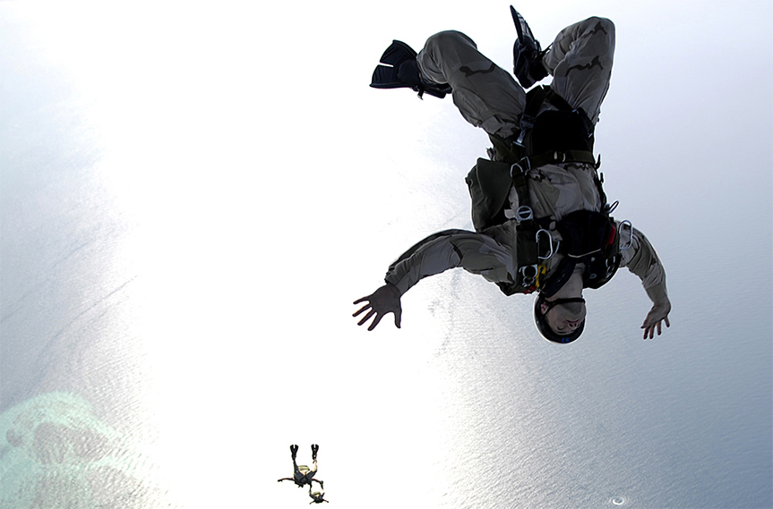
Two skydivers free falling in the sky. — **Figure 4.** Skydivers can adjust the velocity of their dive by changing the position of their body during the free fall. (credit: Jeremy T. Lock)

Julie is an avid skydiver. She has more than 300 jumps under her belt and has mastered the art of making adjustments to her body position in the air to control how fast she falls. If she arches her back and points her belly toward the ground, she reaches a terminal velocity of approximately 120 mph (176 ft/sec). If, instead, she orients her body with her head straight down, she falls faster, reaching a terminal velocity of 150 mph (220 ft/sec).

Since Julie will be moving (falling) in a downward direction, we assume the downward direction is positive to simplify our calculations. Julie executes her jumps from an altitude of 12,500 ft. After she exits the aircraft, she immediately starts falling at a velocity given by $\ds \displaystyle v\left(t\right)=32t.$ She continues to accelerate according to this velocity function until she reaches terminal velocity. After she reaches terminal velocity, her speed remains constant until she pulls her ripcord and slows down to land.

On her first jump of the day, Julie orients herself in the slower “belly down” position (terminal velocity is 176 ft/sec). Using this information, answer the following questions.

How long after she exits the aircraft does Julie reach terminal velocity?
Based on your answer to question 1, set up an expression involving one or more integrals that represents the distance Julie falls after 30 sec.
If Julie pulls her ripcord at an altitude of 3000 ft, how long does she spend in a free fall?
Julie pulls her ripcord at 3000 ft. It takes 5 sec for her parachute to open completely and for her to slow down, during which time she falls another 400 ft. After her canopy is fully open, her speed is reduced to 16 ft/sec. Find the total time Julie spends in the air, from the time she leaves the airplane until the time her feet touch the ground.
On Julie’s second jump of the day, she decides she wants to fall a little faster and orients herself in the “head down” position. Her terminal velocity in this position is 220 ft/sec. Answer these questions based on this velocity:
How long does it take Julie to reach terminal velocity in this case?
Before pulling her ripcord, Julie reorients her body in the “belly down” position so she is not moving quite as fast when her parachute opens. If she begins this maneuver at an altitude of 4000 ft, how long does she spend in a free fall before beginning the reorientation?
Some jumpers wear “wingsuits” (see the picture below). These suits have fabric panels between the arms and legs and allow the wearer to glide around in a free fall, much like a flying squirrel. (Indeed, the suits are sometimes called “flying squirrel suits.”) When wearing these suits, terminal velocity can be reduced to about 30 mph (44 ft/sec), allowing the wearers a much longer time in the air. Wingsuit flyers still use parachutes to land; although the vertical velocities are within the margin of safety, horizontal velocities can exceed 70 mph, much too fast to land safely.

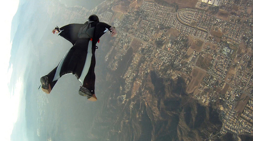
A person falling in a wingsuit, which works to reduce the vertical velocity of a skydiver’s fall. — **Figure 5.** The fabric panels on the arms and legs of a wingsuit work to reduce the vertical velocity of a skydiver’s fall. (credit: Richard Schneider)

Answer the following question based on the velocity in a wingsuit.

If Julie dons a wingsuit before her third jump of the day, and she pulls her ripcord at an altitude of 3000 ft, how long does she get to spend gliding around in the air?

Key Concepts

The Mean Value Theorem for Integrals states that for a continuous function over a closed interval, there is a value c such that $\ds \displaystyle f\left(c\right)$ equals the average value of the function.
The Fundamental Theorem of Calculus, Part 1 shows the relationship between the derivative and the integral.
The Fundamental Theorem of Calculus, Part 2 is a formula for evaluating a definite integral in terms of an antiderivative of its integrand. The total area under a curve can be found using this formula.

Key Equations

Mean Value Theorem for Integrals
If $\ds \displaystyle f\left(x\right)$ is continuous over an interval $\ds \displaystyle \left[a,b\right],$ then there is at least one point $\ds \displaystyle c\in \left[a,b\right]$ such that $\ds \displaystyle f\left(c\right)=\frac{1}{b-a}\int\limits_ {a}^{b}f\left(x\right)\,dx .$
Fundamental Theorem of Calculus Part 1
If $\ds \displaystyle f\left(x\right)$ is continuous over an interval $\ds \displaystyle \left[a,b\right],$ and the function $\ds \displaystyle F\left(x\right)$ is defined by $\ds \displaystyle F\left(x\right)=\int\limits_ {a}^{x}f\left(t\right)dt,$ then $\ds \displaystyle {F}^{\prime }(x)=f\left(x\right).$
Fundamental Theorem of Calculus Part 2
If f is continuous over the interval $\ds \displaystyle \left[a,b\right]$ and $\ds \displaystyle F\left(x\right)$ is any antiderivative of $\ds \displaystyle f\left(x\right),$ then $\ds \displaystyle \int\limits_ {a}^{b}f\left(x\right)\,dx =F\left(b\right)-F\left(a\right).$

Exercises

1. Two mountain climbers start their climb at base camp, taking two different routes, one steeper than the other, and arrive at the peak at exactly the same time. Is it necessarily true that, at some point, both climbers increased in altitude at the same rate?

Answer

Yes. It is implied by the Mean Value Theorem for Integrals.

2. To get on a certain toll road a driver has to take a card that lists the mile entrance point. The card also has a timestamp. When going to pay the toll at the exit, the driver is surprised to receive a speeding ticket along with the toll. Explain how this can happen.

3. Set $\ds \displaystyle F\left(x\right)=\int\limits_ {1}^{x}\left(1-t\right)dt.$ Find $\ds \displaystyle {F}^{\prime }(2)$ and the average value of $\ds \displaystyle {F}'$ over $\ds \displaystyle \left[1,2\right].$

Answer

$\ds \displaystyle {F}^{\prime }(2)=-1;$ average value of $\ds \displaystyle {F}'$ over $\ds \displaystyle \left[1,2\right]$ is $\ds \displaystyle -1\text{/}2.$

In the following exercises, use the Fundamental Theorem of Calculus, Part 1, to find the derivative $\ds\frac{d}{\,dx }\left(f(x)\right)$ of the given function $f$ .

4. $\ds \displaystyle f(x)=\int\limits_ {1}^{x}\sin({-{t}^{2}})dt$

5. $\ds \displaystyle f(x)=\int\limits_ {x}^{0}{e}^{\text{cos}\phantom{\rule{0.1em}{0ex}}(t)}dt$

Answer

$\ds \displaystyle -{e}^{\text{cos}\phantom{\rule{0.1em}{0ex}}(x)}$

6. $\ds \displaystyle f(x)=\int\limits_ {3x}^{1}\sqrt{9-{y}^{2}}dy$

7. $\ds \displaystyle f(x)=\int\limits_ {4}^{\sin(x)}\frac{ds}{\sqrt{16+{s}^{2}}}$

Answer

$\ds \displaystyle \frac{1}{\sqrt{16+\sin^{2}(x)}}\cdot\cos(x)$

8. $\ds \displaystyle f(x)=\int\limits_ {1-x}^{\ln(x)}(\sqrt{t}+t)dt$

9. $\ds \displaystyle f(x)=\int\limits_ {\sqrt e}^{x\sqrt{x}} \frac {t^4}{t+1}dt$

Answer

$\ds \displaystyle \frac{x^6}{x\sqrt x+1}\cdot\frac32 x^{1\text{/}2}$

10. $\ds \displaystyle f(x)=\int\limits_ {\tan^{-1}(x)}^{\tan(x)}t(t+1)dt$

11. $\ds \displaystyle f(x)=\int\limits_ {\cos(2x)}^{\text{sin}\phantom{\rule{0.1em}{0ex}}(x)}\sqrt{1-{t}}dt$

Answer

$\ds \displaystyle \sqrt{1-\sin(x)}\cdot \cos(x)-\sqrt{1-{\text{cos}}(2x)}\cdot(-\sin(2x))\cdot2$

12. $\ds \displaystyle f(x)=\int\limits_ {e^x}^{e^2}\frac{\ln(t)}{1+{t}}dt$

13. $\ds \displaystyle f(x)=\int\limits_ {\sqrt[3]{x^2}}^{x}(2t^6+5)dt$

Answer

$\ds \displaystyle 2x^6+5-(2x^4+5)\cdot \frac23 x^{-1\text{/}3}$

14. $\ds \displaystyle f(x)=\int\limits_ {x}^{\text{ln}\phantom{\rule{0.1em}{0ex}}(1+x)}e^{\sec(2t)}dt$

15. $\ds \displaystyle f(x)=\int\limits_ {\pi^2}^{y^{4}}\sin(\sqrt u)du$

( Hint: does the function depend on $x$ ?)

Answer

$\ds \displaystyle 0$

16. The graph of $\ds \displaystyle y=\int\limits_ {0}^{x}f\left(t\right)dt,$ where f is a piecewise constant function, is shown here.

A function with linear segments which goes through the points (0, 0), (1, 3), (2, 2), (3, 0), (4, 3), (5, 3), and (6, 2). The area under the function and above the x axis is shaded.

Over which intervals is f positive? Over which intervals is it negative? Over which intervals, if any, is it equal to zero?
What are the maximum and minimum values of f?
What is the average value of f?

17. The graph of $\ds \displaystyle y=\int\limits_ {0}^{x}f\left(t\right)dt,$ where f is a piecewise constant function, is shown here.

A graph of a function with linear segments that goes through the points (0, 0), (1, -1), (2, 1), (3, 1), (4, -2), (5, -2), and (6, 0). The area over the function but under the x axis over the interval [0, 1.5] and [3.25, 6] is shaded. The area under the function but over the x axis over the interval [1.5, 3.25] is shaded.

Over which intervals is f positive? Over which intervals is it negative? Over which intervals, if any, is it equal to zero?
What are the maximum and minimum values of f?
What is the average value of f?

Answer

a. f is positive over $\ds \displaystyle \left[1,2\right]$ and $\ds \displaystyle \left[5,6\right],$ negative over $\ds \displaystyle \left[0,1\right]$ and $\ds \displaystyle \left[3,4\right],$ and zero over $\ds \displaystyle \left[2,3\right]$ and $\ds \displaystyle \left[4,5\right].$ b. The maximum value is 2 and the minimum is −3. c. The average value is 0.

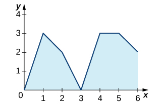
18. The graph of $\ds \displaystyle y=\int\limits_ {0}^{x}\ell \left(t\right)dt,$ where ℓ is a piecewise linear function, is shown here.

A graph of a function which goes through the points (0, 0), (1, -1), (2, 1), (3, 3), (4, 3.5), (5, 4), and (6, 2). The area over the function and under the x axis over [0, 1.8] is shaded, and the area under the function and over the x axis is shaded.

Over which intervals is ℓ positive? Over which intervals is it negative? Over which, if any, is it zero?
Over which intervals is ℓ increasing? Over which is it decreasing? Over which, if any, is it constant?
What is the average value of ℓ?

19. The graph of $\ds \displaystyle y=\int\limits_ {0}^{x}\ell \left(t\right)dt,$ where ℓ is a piecewise linear function, is shown here.

A graph of a function that goes through the points (0, 0), (1, 1), (2, 0), (3, -1), (4.5, 0), (5, 1), and (6, 2). The area under the function and over the x axis over the intervals [0, 2] and [4.5, 6] is shaded. The area over the function and under the x axis over the interval [2, 2.5] is shaded.

Over which intervals is ℓ positive? Over which intervals is it negative? Over which, if any, is it zero?
Over which intervals is ℓ increasing? Over which is it decreasing? Over which intervals, if any, is it constant?
What is the average value of ℓ?

Answer

a. ℓ is positive over $\ds \displaystyle \left[0,1\right]$ and $\ds \displaystyle \left[3,6\right],$ and negative over $\ds \displaystyle \left[1,3\right].$ b. It is increasing over $\ds \displaystyle \left[0,1\right]$ and $\ds \displaystyle \left[3,5\right],$ and it is constant over $\ds \displaystyle \left[1,3\right]$ and $\ds \displaystyle \left[5,6\right].$ c. Its average value is $\ds \displaystyle \frac{1}{3}.$

In the following exercises, use basic integration formulas to compute the given indefinite integral.

20. $\ds \ds\int \left(x^2-7x+2\right)\,dx$

21. $\ds \ds\int \left(x^3+\frac4{x^3}\right)\,dx$

Answer

$\ds \ds\frac{1}{4}{x}^{4}-2{x}^{-2}+C$

22.

$\ds \ds\int \left(\frac ex+\pi^2\right)\,dx$

23. $\ds \ds\int \left(\sqrt{x}-\frac{1}{\sqrt{x}}\right)\,dx$

Answer

$\ds \ds\frac{2}{3}{x}^{3\text{/}2}-2{x}^{1\text{/}2}+C$

24. $\ds \ds\int \left(x^2-\frac3x\right)\left(\frac1x+1\right)\,dx$

25. $\ds \ds\int\frac{{5}^{x}-{2}^{x}}{3}\,dx$

Answer

$\ds \ds\frac{5^x}{3\ln(5)}-\frac{2^x}{3\ln(2)}+C$

26. $\ds \ds\int (\pi\sin(x)-\csc^2(x))\,dx$

In the following exercises, evaluate each definite integral using the Fundamental Theorem of Calculus, Part 2.

27. $\ds \displaystyle \int\limits_ {-2}^{3}\left({x}^{2}+3x-5\right)\,dx$

Answer

$\ds \displaystyle F\left(x\right)=\frac{{x}^{3}}{3}+\frac{3{x}^{2}}{2}-5x,F\left(3\right)-F\left(-2\right)=-\frac{35}{6}$

28. $\ds \displaystyle \int\limits_ {-1}^{1}\left(t+2\right)\left(t-3\right)dt$

29. $\ds \displaystyle \int\limits_ {2}^{3}\left({t}^{2}-9\right)\left(4-{t}^{2}\right)dt$

Answer

$\ds \displaystyle F\left(t\right)=-\frac{{t}^{5}}{5}+\frac{13{t}^{3}}{3}-36t,F\left(3\right)-F\left(2\right)=\frac{62}{15}$

30. $\ds \displaystyle \int\limits_ {1}^{2}\frac{1+2x}{\sqrt x}\,dx$

31. $\ds \displaystyle \int\limits_ {0}^{1}x\left(\sqrt{x^3}-2\right)\,dx$

Answer

$\ds \displaystyle F\left(x\right)=\frac27x^{7\text{/}2}-x^2,F\left(1\right)-F\left(0\right)=-\frac57$

32. $\ds \displaystyle \int\limits_ {4}^{9}\left(t^{1\text{/}2}+2\right)^2dt$

33. $\ds \displaystyle \int\limits_ {1\text{/}4}^{1}\left(\frac3x+\frac{2}{{x}^{2}}\right)\,dx$

Answer

$\ds \displaystyle F\left(x\right)=3\ln|x|-\frac{2}{x},F\left(1\right)-F\left(\frac{1}{4}\right)=6+3\ln(4)$

34. $\ds \displaystyle \int\limits_ {-1}^{0}(3^x-e^3)\,dx$

35. $\ds \displaystyle \int\limits_ {0}^{1}(e^x+x^e)\,dx$

Answer

$\ds \displaystyle F\left(x\right)=e^x+\frac{x^{e+1}}{e+1},F\left(1\right)-F\left(0\right)=e-1+\frac1{e+1}$

36. $\ds \displaystyle \int\limits_ {\pi\text{/}3}^{\pi\text{/}2}\sin(t)dt$

37. $\ds \displaystyle \int\limits_ {0}^{\pi\text{/}4}\sec(x)\cos^2(x)\,dx$

(Hint: express the integrand in terms of $\sin(x)$ and $\cos(x)$ )

Answer

$\ds \displaystyle F\left(x\right)=\sin(x),F\left(\pi\text{/}4\right)-F\left(0\right)=\frac{\sqrt2}{2}$

38. $\ds \displaystyle \int\limits_ {2\pi \text{/}3}^{\pi}\frac{1}{\cos^2(\theta)} d\theta$

(Hint: rewrite the integrand in terms of another trigonometric function.)

39. $\ds \displaystyle \int\limits_ {0}^{\pi \text{/}6}\sin(\theta)\big(2-\cot(\theta)\big)d\theta$

Answer

$\ds \displaystyle F\left(\theta\right)=-2\cos(\theta)-\sin(\theta), F\left(\pi\text{/}6\right)-F\left(0\right)=-\sqrt3+\frac32$

40. $\ds \displaystyle \int\limits_ {-\pi\text{/}4}^{0}\frac{1-\sin(\theta)}{\cos^2(\theta)} d\theta$

(Hint: split the numerator and rewrite the integrand in terms of $\sec(\theta)$ and $\tan(\theta)$ )

41. $\ds \displaystyle \int\limits_ {\pi \text{/}3}^{\pi \text{/}2} \cot^2(t)dt$

(Hint: express the integrand in terms of $\csc(t)$ )

Answer

$\ds \displaystyle F\left(t\right)=-\cot(t)-t, F\left(\frac{\pi }{2}\right)-F\left(\frac{\pi}3\right)=\frac{\sqrt3}3-\frac{\pi}6$

42. $\ds \displaystyle \int\limits_ {-e}^{-1} \frac{2t+3}tdt$

43. $\ds \displaystyle \int\limits_{1\text{/}2}^{\sqrt2\text{/}2} \frac2{\sqrt{1-x^2}}\,dx$

Answer

$\ds \displaystyle F\left(x\right)=2\sin^{-1}(x), F\left(\frac{\sqrt2}{2}\right)-F\left(\frac12\right)=\frac{\pi}6$

In the following exercises, use the evaluation theorem (Fundamental Theorem of Calculus, Part 2) to express the given integral as an explicit function of $x$ .

44. $\ds \displaystyle \int\limits_ {a}^{x}\frac1{t^3}dt$

45. $\ds \displaystyle \int\limits_ {1}^{x}\frac1{2t^2+2}dt$

Answer

$\ds \displaystyle\frac12\tan^{-1}(x)-\frac{\pi}8$

46. $\ds \displaystyle \int\limits_ {\pi\text{/}2}^{2x} \csc(t)\cot(t)dt$

47. $\ds \displaystyle \int\limits_ {-x}^{x}\text{sin}\phantom{\rule{0.1em}{0ex}}(t)dt$

Answer

$\ds \displaystyle0$

In the following exercises, identify the roots of the integrand to remove absolute values, then evaluate using the Fundamental Theorem of Calculus, Part 2.

48. $\ds \displaystyle \int\limits_ {-2}^{3}|x|\,dx$

49. $\ds \displaystyle \int\limits_ {-2}^{4}|{t}^{2}-2t-3|dt$

Answer

$\ds \displaystyle \int\limits_ {-2}^{-1}\left({t}^{2}-2t-3\right)dt-\int\limits_ {-1}^{3}\left({t}^{2}-2t-3\right)dt+\int\limits_ {3}^{4}\left({t}^{2}-2t-3\right)dt=\frac{46}{3}$

50. $\ds \displaystyle \int\limits_ {0}^{\pi }|\text{cos}\phantom{\rule{0.1em}{0ex}}(t)|dt$

51. $\ds \displaystyle \int\limits_ {-\pi \text{/}2}^{\pi \text{/}2}|\text{sin}\phantom{\rule{0.1em}{0ex}}(t)|dt$

Answer

$\ds \displaystyle -\int\limits_ {-\pi \text{/}2}^{0}\text{sin}\phantom{\rule{0.1em}{0ex}}(t)dt+\int\limits_ {0}^{\pi \text{/}2}\text{sin}\phantom{\rule{0.1em}{0ex}}(t)dt=2$

52. Explain why, if f is continuous over $\ds \displaystyle \left[a,b\right]$ and is not equal to a constant, there is at least one point $\ds \displaystyle c\in \left[a,b\right]$ such that $\ds \displaystyle f\left(c\right)=\frac{1}{b-a}\int\limits_ {a}^{b}f\left(t\right)dt$ and at least one point $\ds \displaystyle d\in \left[a,b\right]$ such that $\ds \displaystyle f\left(d\right)<\frac{1}{b-a}\int\limits_ {a}^{b}f\left(t\right)dt.$

(Hint: If f is not constant, then its average is strictly smaller than the maximum and larger than the minimum, which are attained over $\ds \displaystyle \left[a,b\right]$ by the extreme value theorem.)

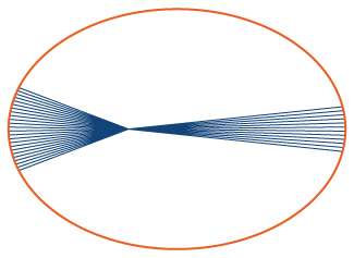
53. Kepler’s first law states that the planets move in elliptical orbits with the Sun at one focus. The closest point of a planetary orbit to the Sun is called the perihelion (for Earth, it currently occurs around January 3) and the farthest point is called the aphelion (for Earth, it currently occurs around July 4). Kepler’s second law states that planets sweep out equal areas of their elliptical orbits in equal times. Thus, the two arcs indicated in the following figure are swept out in equal times. At what time of year is Earth moving fastest in its orbit? When is it moving slowest?

A horizontal ellipse with one focus marked. Two equal arcs are marked to the direct left of the focus and on the other side of the ellipse. The wedges formed by the focus and the endpoints of both arcs are shaded in blue.

54. A point on an ellipse with major axis length 2a and minor axis length 2b has the coordinates $\ds \displaystyle \left(a\phantom{\rule{0.1em}{0ex}}\text{cos}\phantom{\rule{0.1em}{0ex}}(\theta) ,b\phantom{\rule{0.1em}{0ex}}\text{sin}\phantom{\rule{0.1em}{0ex}}(\theta) \right),0\le \theta \le 2\pi .$

Show that the distance from this point to the focus at $\ds \displaystyle \left(-c,0\right)$ is $\ds \displaystyle d\left(\theta \right)=a+c\phantom{\rule{0.1em}{0ex}}\text{cos}\phantom{\rule{0.1em}{0ex}}(\theta) ,$ where $\ds \displaystyle c=\sqrt{{a}^{2}-{b}^{2}}.$
Use these coordinates to show that the average distance $\ds \displaystyle \overline{d}$ from a point on the ellipse to the focus at $\ds \displaystyle \left(-c,0\right),$ with respect to angle θ, is a.

Answer

a. $\ds \displaystyle {d}^{2}(\theta) ={\left(a\phantom{\rule{0.1em}{0ex}}\text{cos}\phantom{\rule{0.1em}{0ex}}(\theta) +c\right)}^{2}+{b}^{2}{\text{sin}}^{2}(\theta) ={a}^{2}+{c}^{2}{\text{cos}}^{2}(\theta) +2ac\cdot\phantom{\rule{0.1em}{0ex}}\text{cos}\phantom{\rule{0.1em}{0ex}}(\theta)$ $\ds ={\left(a+c\phantom{\rule{0.1em}{0ex}}\text{cos}\phantom{\rule{0.1em}{0ex}}(\theta) \right)}^{2},$ and so $d(\theta)=|a+c\cos(\theta)|=a+c\cos(\theta)$ since $a+c\cos(\theta)\ge a-c=a-\sqrt{a^2-b^2}\ge0$ .

b. $\ds \displaystyle \stackrel{-}{d}=\frac{1}{2\pi }\int\limits_ {0}^{2\pi }\left(a+c\phantom{\rule{0.1em}{0ex}}\text{cos}\phantom{\rule{0.1em}{0ex}}(\theta) \right)d(\theta) =a$

55. As implied earlier, according to Kepler’s laws, Earth’s orbit is an ellipse with the Sun at one focus. The perihelion for Earth’s orbit around the Sun is 147,098,290 km and the aphelion is 152,098,232 km.

By placing the major axis along the x-axis, find the average distance from Earth to the Sun.
The classic definition of an astronomical unit (AU) is the distance from Earth to the Sun, and its value was computed as the average of the perihelion and aphelion distances. Is this definition justified?

56. The force of gravitational attraction between the Sun and a planet is $\ds \displaystyle F\left(\theta \right)=\frac{GmM}{{r}^{2}\left(\theta \right)},$ where m is the mass of the planet, M is the mass of the Sun, G is a universal constant, and $\ds \displaystyle r\left(\theta \right)$ is the distance between the Sun and the planet when the planet is at an angle θ with the major axis of its orbit. Assuming that M, m, and the ellipse parameters a and b (half-lengths of the major and minor axes) are given, set up—but do not evaluate—an integral that expresses in terms of $\ds \displaystyle G,m,M,a,b$ the average gravitational force between the Sun and the planet.

Answer

Mean gravitational force = $\ds \displaystyle \frac{GmM}{2}\int\limits_ {0}^{2\pi }\frac{1}{{\left(a+2\sqrt{{a}^{2}-{b}^{2}}\text{cos}\phantom{\rule{0.1em}{0ex}}\theta \right)}^{2}}d\theta .$

57. The displacement from rest of a mass attached to a spring satisfies the simple harmonic motion equation $\ds \displaystyle x\left(t\right)=A\phantom{\rule{0.1em}{0ex}}\text{cos}\left(\omega t-\varphi \right),$ where $\ds \displaystyle \varphi$ is a phase constant, ω is the angular frequency, and A is the amplitude. Find the average velocity, the average speed (magnitude of velocity), the average displacement, and the average distance from rest (magnitude of displacement) of the mass.

Glossary

fundamental theorem of calculus: the theorem, central to the entire development of calculus, that establishes the relationship between differentiation and integration

fundamental theorem of calculus, part 1: uses a definite integral to define an antiderivative of a function

fundamental theorem of calculus, part 2: (also, evaluation theorem) we can evaluate a definite integral by evaluating the antiderivative of the integrand at the endpoints of the interval and subtracting

mean value theorem for integrals: guarantees that a point c exists such that $\ds \displaystyle f\left(c\right)$ is equal to the average value of the function

License

Icon for the Creative Commons Attribution-NonCommercial-ShareAlike 4.0 International License

Calculus: Volume 2 (Second University of Manitoba Edition) Copyright © 2021 by Gilbert Strang and Edward 'Jed' Herman, modified by Varvara Shepelska is licensed under a Creative Commons Attribution-NonCommercial-ShareAlike 4.0 International License, except where otherwise noted.

Learning Objectives

The Mean Value Theorem for Integrals

The Mean Value Theorem for Integrals

Proof

Finding the Average Value of a Function

Solution

Answer

Fundamental Theorem of Calculus Part 1: Integrals and Antiderivatives

Fundamental Theorem of Calculus, Part 1

Proof

Finding a Derivative with the Fundamental Theorem of Calculus

Solution

Answer

Using the Fundamental Theorem and the Chain Rule to Calculate Derivatives

Solution

Answer

Using the Fundamental Theorem of Calculus with Two Variable Limits of Integration

Solution

Answer

Antiderivatives and Indefinite Integrals

Definition

Properties of Indefinite Integrals

Evaluating Indefinite Integrals

Solution

Answer

Fundamental Theorem of Calculus, Part 2: The Evaluation Theorem

The Fundamental Theorem of Calculus, Part 2

Proof

Evaluating an Integral with the Fundamental Theorem of Calculus

Solution

Analysis

Evaluating a Definite Integral Using the Fundamental Theorem of Calculus, Part 2

Solution

Answer

A Roller-Skating Race

Solution

Answer

A Parachutist in Free Fall

Key Concepts

Key Equations

Exercises

Answer

Answer

Answer

Answer

Answer

Answer

Answer

Answer

Answer

Answer

Answer

Answer

Answer

Answer

Answer

Answer

Answer

Answer

Answer

Answer

Answer

Answer

Answer

Answer

Answer

Answer

Answer

Answer

Glossary

License

Share This Book