7.2 Calculus of Parametric Curves
Learning Objectives
- Determine derivatives and equations of tangents for parametric curves.
- Find the area under a parametric curve.
- Determine the arc length of a parametric curve.
- Apply the formula for the surface area of the surface generated by revolving a parametric curve about the x-axis or the y-axis.
Now that we have introduced the concept of a parameterized curve, our next step is to learn how to work with this concept in the context of calculus. For example, if we know a parameterization of a given curve, is it possible to calculate the slope of a tangent line to the curve? How about the arc length of the curve? Or the area under the curve?
Another scenario: Suppose we would like to represent the location of a baseball after the ball leaves a pitcher’s hand. If the position of the baseball is represented by the plane curve  then we should be able to use calculus to find the speed of the ball at any given time. Furthermore, we should be able to calculate just how far that ball has traveled as a function of time.
Derivatives of Parametric Equations
We start by asking how to calculate the slope of a line tangent to a parametric curve at a point. Consider the plane curve defined by the parametric equations

The graph of this curve appears in Figure 1 below. It is a line segment starting at  and ending at
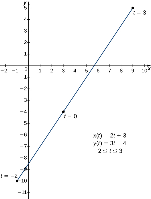
We can eliminate the parameter by first solving the equation  for t:
![\ds \begin{array}{ccc}\hfill x\left(t\right)&\ds =\hfill &\ds 2t+3\hfill \\[5mm]\ds \hfill x-3&\ds =\hfill &\ds 2t\hfill \\[5mm]\ds \hfill t&\ds =\hfill &\ds \frac{x-3}{2}.\hfill \end{array}](https://pressbooks.openedmb.ca/app/uploads/quicklatex/quicklatex.com-1aad1e1df9b2c7c940cae20cde6f0a23_l3.png "Rendered by QuickLaTeX.com")
Substituting this into  we obtain
![\ds \begin{array}{ccc}\hfill y\left(t\right)&\ds =\hfill &\ds 3t-4\hfill \\[5mm]\ds \hfill y&\ds =\hfill &\ds 3\left(\frac{x-3}{2}\right)-4\hfill \\[5mm]\ds \hfill y&\ds =\hfill &\ds \frac{3x}{2}-\frac{9}{2}-4\hfill \\[5mm]\ds \hfill y&\ds =\hfill &\ds \frac{3x}{2}-\frac{17}{2}.\hfill \end{array}](https://pressbooks.openedmb.ca/app/uploads/quicklatex/quicklatex.com-de751983656bdf9b5a8d11cd44682416_l3.png "Rendered by QuickLaTeX.com")
The slope of this line is given by  Next we calculate
  and
and  This gives
  and
and  Notice that
  This is no coincidence, as outlined in the following theorem.
Derivative of Parametric Equations
Consider the plane curve defined by the parametric equations  and
and  Suppose that and
  exist, and assume that
  Then the derivative
  is given by

Proof
This theorem can be proven using the Chain Rule. In particular, assume that the parameter t can be eliminated, yielding a differentiable function  Then
Then  Differentiating both sides of this equation using the Chain Rule yields
 so
so

But  which proves the theorem. □
The formula (*) from the previous theorem can be used to calculate the first derivative for a curve defined parametrically at the given value  of
of  , and hence the slope of the tangent line to the curve at the point
  corresponding to
  . For the purpose of sketching parametric curves, it is useful to determine, where the tangent to the curve is horizontal and where it is vertical. It has a direct analogy with considering the critical points on the graph of a curve with explicit equation
  , corresponding to the values
  of
of  , such that
  or
or  is undefined. Based on (*), we see that the tangent to the parametric curve
  ,
,  is horizontal where
  and
and  , and the tangent is vertical where
  and
and  .
.
Finding the Derivative for a Parametric Curve
For each of the following parametrically defined plane curves, calculate the derivative  as well as determine the points, where the tangent line is horizontal and the points, where the tangent line is vertical.


Solution
- To apply (*), first calculate
 and
and 

Next substitute these into (*):

Since
, there are no points on the curve, where the tangent line is horizontal. Solving  , we find the value of
  corresponding to the point on the curve, where the tangent line is vertical. Calculating
  and
and  gives
gives  and
and  yielding the point
  on the curve. Note that, eliminating the parameter, we can determine that this curve is a parabola opening to the right, and the point is its vertex as shown below.
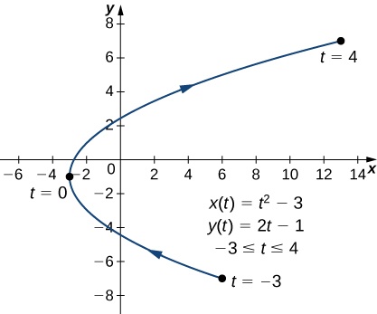
Figure 2. Graph of the parabola described by parametric equations in part a. - Again, we start by calculating and

Next substitute these into (*) to find
 :
:

Since
, there are no points on this curve, where the tangent line is vertical. To determine the points, where the tangent line is horizontal, we solve  , and find that
  . When
  ,
,  and
and  which corresponds to the point
  on the curve. When
  ,
, and
and  which corresponds to the point
 on the curve. The following figure provides the sketch of the curve.
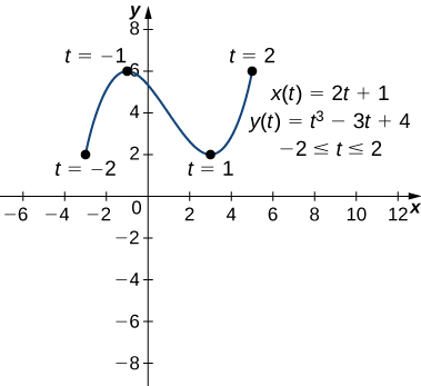
Figure 3. Graph of the curve described by parametric equations in part b. - Calculating and
 we obtain

Therefore, (*) yields

We see that
 when
when  in the interval
 ![\ds[0,2\pi]](https://pressbooks.openedmb.ca/app/uploads/quicklatex/quicklatex.com-0c6bb6eacbc7af9f38cfefea098cfe17_l3.png "Rendered by QuickLaTeX.com") . Note that
. Note that  and
and  .
.Hence, each of these values of
yields a point on the curve, where the tangent line is horizontal. To find the coordinates of these points, we substitute  and
and  into
into  and
and  :
:  ,
,  , yielding the point
  , and
, and  ,
,  , yielding the point
  .
. Solving
 , we find
  within
 ![[0,2\pi]](https://pressbooks.openedmb.ca/app/uploads/quicklatex/quicklatex.com-ce20c94fe55da7e7ed58648120072837_l3.png "Rendered by QuickLaTeX.com") . Since
. Since  is non-zero at all these values of , each of them corresponds to a point on the curve, where the tangent line is vertical. Substituting into and , we find the coordinates of these points to be
  ,
,  and respectively.
 The above computations agree with the sketch of the parametric curve, which is a circle of radius 5 with the center at the origin.
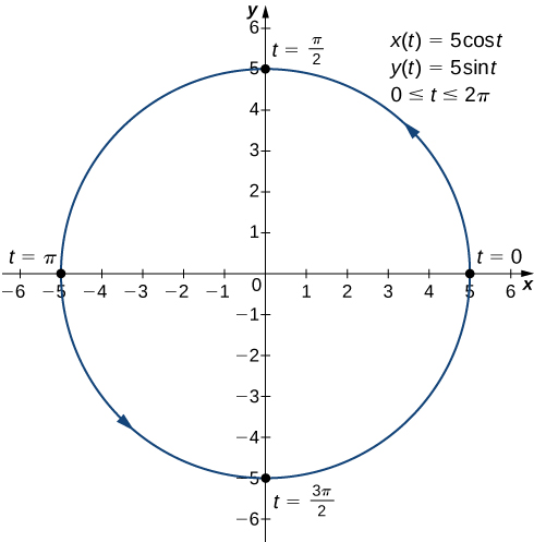
Figure 4. Graph of the curve described by parametric equations in part c.
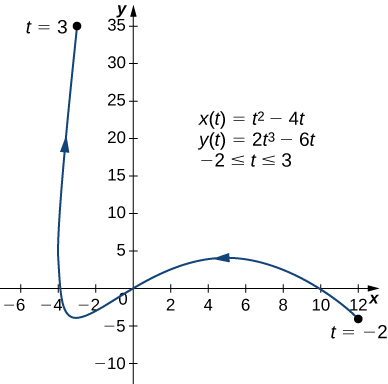
Calculate the derivative  for the curve defined by the parametric equations
 ,
,  and find all points on the curve, where the tangent line is horizontal or where the tangent line is vertical.
Answer

The tangent line line is horizontal at  and
and  , corresponding to
  and
and  respectively. The tangent line is vertical at
  , corresponding to
  .
.
Slope of the Tangent Line in a Special Case
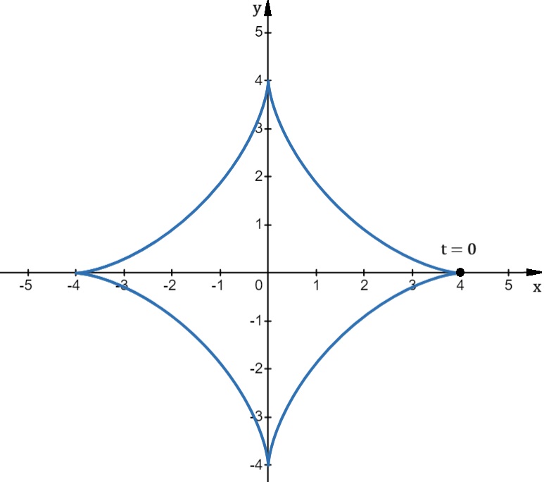
Determine the slope of the tangent line to the hypocycloid


Solution
We first calculate and 

We see that  , and so (*) cannot be applied to find
  when
when  . However,
  when
when ![t\in\left[-\dfrac{\pi}6,\dfrac{\pi}6\right]\setminus\{0\}](https://pressbooks.openedmb.ca/app/uploads/quicklatex/quicklatex.com-0023f204c96113b624efe13f85977bdd_l3.png "Rendered by QuickLaTeX.com") ,
, ![\left(x'(t)>0 \text{ when } t\in\left[-\dfrac{\pi}6,0\right)\text{ and }x'(t)<0 \text{ when } t\in\left(0,\dfrac{\pi}6\right]\right)](https://pressbooks.openedmb.ca/app/uploads/quicklatex/quicklatex.com-eba73e08b789f68f84552fd253e92e70_l3.png "Rendered by QuickLaTeX.com") , and so we can consider
, and so we can consider  :
:

Since  we deal with a
  indeterminate form and can apply L’Hospital’s rule.
![\ds \begin{array}{ccc}\hfill \lim\limits_{t\to0} \dfrac{dy}{dx}&\ds =\hfill &\ds \lim\limits_{t\to0} \dfrac{3\cos(t)-3\cos(3t)}{-3\sin(t)-3\sin(3t)}\hfill \\[5mm]\ds \hfill &\ds =\hfill &\ds \lim\limits_{t\to0} \dfrac{-3\sin(t)+9\sin(3t)}{-3\cos(t)-9\cos(3t)}\hfill \\[5mm]\ds \hfill &\ds =\hfill &\ds \dfrac{-0+0}{-3-9}=\frac{0}{-12}=0.\hfill \end{array}](https://pressbooks.openedmb.ca/app/uploads/quicklatex/quicklatex.com-43d16cd120ab3e3ffa9cf556405dc0e5_l3.png "Rendered by QuickLaTeX.com")
Therefore, when , the slope of the tangent line is zero, and hence the tangent line to the hypocycloid is horizontal at the point  , corresponding to , where the curve has a cusp.
Finding a Tangent Line
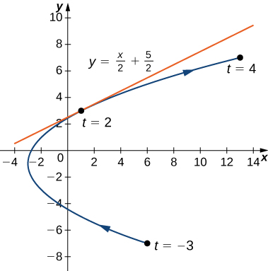
Find the equation of the tangent line to the parametric curve defined by the equations


Solution
We first calculate and

Next we substitute these into (*):

When 
 so this is the slope of the tangent line. Calculating
  and
and  gives
gives  and
and  which corresponds to the point
  on the curve, see Figure 5 below. We now use the point-slope form of the equation of a line to find the equation of the tangent line at this point:
![\ds \begin{array}{ccc}\hfill y-{y}_{0}&\ds =\hfill &\ds m\left(x-{x}_{0}\right)\hfill \\[5mm]\ds \hfill y-3&\ds =\hfill &\ds \frac{1}{2}\left(x-1\right)\hfill \\[5mm]\ds \hfill y-3&\ds =\hfill &\ds \frac{1}{2}x-\frac{1}{2}\hfill \\[5mm]\ds \hfill y&\ds =\hfill &\ds \frac{1}{2}x+\frac{5}{2}.\hfill \end{array}](https://pressbooks.openedmb.ca/app/uploads/quicklatex/quicklatex.com-13c3bba2efea03dec74b5fdaa106dfb0_l3.png "Rendered by QuickLaTeX.com")

Find the equation of the tangent line to the curve defined by the equations


Answer
The equation of the tangent line is 
Second-Order Derivatives
Our next goal is to see how to take the second derivative of a function defined parametrically. The second derivative of a function  is defined to be the derivative of the first derivative; that is,
![\ds \frac{{d}^{2}y}{d{x}^{2}}=\frac{d}{\,dx }\left[\frac{dy}{\,dx }\right].](https://pressbooks.openedmb.ca/app/uploads/quicklatex/quicklatex.com-5aca1da9d088c73c59f705f01bc056f4_l3.png "Rendered by QuickLaTeX.com")
Since  we can replace the
  on both sides of this equation with
  This gives us

If we know as a function of t, then this formula is straightforward to apply.

 Applying
Calculate the second derivative  for the plane curve defined by the equations
 .
.Answer

From before, we know that the second derivative is “responsible” for concavity of the curve with an explicit equation : the curve is concave upward where  , and it is concave downward where
  Since, locally, a parametric curve usually admits eliminating the parameter and obtaining an explicit equation, we can still look at the sign of
  , to determine where the curve is concave upward and where it is concave downward. Because, in practice, we won't be finding an explicit equation of the curve, but we will be using (**) to find as a function of , it is the intervals in terms of that we will be referring to when discussing concavity of parametric curves.
Examining Concavity of a Parametric Curve
Determine where the parametric curve  ,
,  is concave upward and where it is concave downward.
Solution
Applying (*), we find that  Using (**) together with the quotient rule, we obtain

We now need to determine for which values of , is positive, and for which values of it is negative. Factoring the numerator and denominator, we rewrite :
 .
. The numerator has zeros and  , while the denominator has a zero of multiplicity 3. Using sample points or any other appropriate method, we find that
  , and hence the parametric curve is concave upward, when
  and
and  , and
, and  , implying that the curve is concave downward, when
  and
and  .
.
Determine where the parametric curve  ,
,  is concave upward.
Answer
The curve is concave upward when .
Integrals Involving Parametric Equations
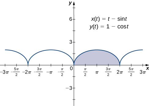
Now that we have seen how to calculate the derivative of a plane curve, the next question is this: How do we find the area under a curve defined parametrically? Recall the cycloid defined by the equations  Suppose we want to find the area of the shaded region in the following graph.
![\ds \left[0,2\pi \right]](https://pressbooks.openedmb.ca/app/uploads/quicklatex/quicklatex.com-d4c3e07b5e02fe7225629a67ce93c5d7_l3.png "Rendered by QuickLaTeX.com") highlighted.
highlighted.To derive a formula for the area under the curve defined by the functions

we assume that  is increasing and differentiable and start with an equal partition of the interval
  Suppose
  and consider the following graph.
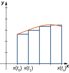
We use rectangles to approximate the area under the curve. The height of a typical rectangle in this parametrization is  for some value
  in the ith subinterval, and the width can be calculated as
  . It follows that the area of the ith rectangle is given by

Then a Riemann sum for the area is

Multiplying and dividing each area by  gives
gives

Taking the limit as  approaches infinity, we obtain

Note that if is decreasing, that is, the curve is traced from left to right, everything in the above derivation stays the same except that the width of a typical rectangle becomes  , which results in the formula

This leads to the following theorem.
Area under a Parametric Curve
Consider the plane curve defined by the parametric equations

and assume that is differentiable.
- If is increasing, then the area under this curve is given by

-
If
is decreasing, then the area under this curve is given by
Finding the Area under a Parametric Curve
Find the area under one arc of the cycloid defined by the equations

Solution
To determine whether is increasing or decreasing we look at the sign of  . We have that
  , and hence is increasing. Applying the above theorem, we have
![\ds \begin{array}{cc}\ds \hfill A&\ds =\int\limits_{a}^{b}y\left(t\right){x}^{\prime }\left(t\right)\phantom{\rule{0.2em}{0ex}}dt\hfill \\[5mm]\ds &\ds =\int\limits_{0}^{2\pi }\left(1-\text{cos}\phantom{\rule{0.2em}{0ex}}(t)\right)\left(1-\text{cos}\phantom{\rule{0.2em}{0ex}}(t)\right)\phantom{\rule{0.2em}{0ex}}dt\hfill \\[5mm]\ds &\ds =\int\limits_{0}^{2\pi }\left(1-2\phantom{\rule{0.2em}{0ex}}\text{cos}\phantom{\rule{0.2em}{0ex}}(t)+{\text{cos}}^{2}(t)\right)dt\hfill \\[5mm]\ds &\ds =\int\limits_{0}^{2\pi }\left(1-2\phantom{\rule{0.2em}{0ex}}\text{cos}\phantom{\rule{0.2em}{0ex}}(t)+\frac{1+\text{cos}\phantom{\rule{0.2em}{0ex}}(2t)}{2}\right)\phantom{\rule{0.2em}{0ex}}dt\hfill \\[5mm]\ds &\ds =\int\limits_{0}^{2\pi }\left(\frac{3}{2}-2\phantom{\rule{0.2em}{0ex}}\text{cos}\phantom{\rule{0.2em}{0ex}}(t)+\frac{\text{cos}\phantom{\rule{0.2em}{0ex}}(2t)}{2}\right)\phantom{\rule{0.2em}{0ex}}dt\hfill \\[5mm]\ds &\ds =\left({\frac{3t}{2}-2\phantom{\rule{0.2em}{0ex}}\text{sin}\phantom{\rule{0.2em}{0ex}}(t)+\frac{\text{sin}\phantom{\rule{0.2em}{0ex}}(2t)}{4}}\right)\Big|_{0}^{2\pi }\hfill \\[5mm]\ds &\ds =3\pi .\hfill \end{array}](https://pressbooks.openedmb.ca/app/uploads/quicklatex/quicklatex.com-fd7a50aa5dc4aaf55760761bda4f6160_l3.png "Rendered by QuickLaTeX.com")
Find the area under the upper half of the hypocycloid defined by the equations

Answer

Hint
Use the above theorem, along with the identities ![\ds \text{sin}\phantom{\rule{0.2em}{0ex}}(\alpha) \phantom{\rule{0.2em}{0ex}}\text{sin}\phantom{\rule{0.2em}{0ex}}(\beta) =\frac{1}{2}\left[\text{cos}\left(\alpha -\beta \right)-\text{cos}\left(\alpha +\beta \right)\right]](https://pressbooks.openedmb.ca/app/uploads/quicklatex/quicklatex.com-0744da7ff713688c5d4ef18ab1dc4f2a_l3.png "Rendered by QuickLaTeX.com") and
and  Note that is decreasing.
Arc Length of a Parametric Curve
The same way we did for a regular curve with explicit equation or  , to derive a formula for the arc length of a parametric curve, we approximate it by a union of line segments as shown in the following figure.
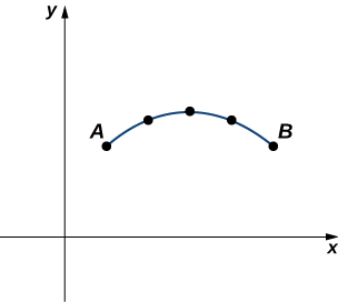
Given a plane curve defined by the parametric equations  we start by partitioning the interval
 ![\ds \left[a,b\right]](https://pressbooks.openedmb.ca/app/uploads/quicklatex/quicklatex.com-c3ac37860878a36cf1c719379b6192f8_l3.png "Rendered by QuickLaTeX.com") into n equal subintervals:
into n equal subintervals:  The width of each subinterval is
  The length of the
  th line segment can be found as follows:

Adding those from  , we obatin an approximation of the arc length s of the parametric curve:

If we assume that and  are differentiable functions of t, then the Mean Value Theorem applies, so in each subinterval
 ![\ds \left[{t}_{k-1},{t}_{k}\right]](https://pressbooks.openedmb.ca/app/uploads/quicklatex/quicklatex.com-35f2258c72c43ba949ccf71a46009783_l3.png "Rendered by QuickLaTeX.com") there exist
there exist  and
and  such that
![\ds \begin{array}{ll}\ds \ds \\[5mm]\ds x\left({t}_{i}\right)-x\left({t}_{i-1}\right)={x}^{\prime }\left(t^*_{i}\right)\left({t}_{i}-{t}_{i-1}\right)={x}^{\prime }\left(t^*_{i}\right)\Delta t\hfill \\[5mm]\ds y\left({t}_{i}\right)-y\left({t}_{i-1}\right)={y}^{\prime }\left(t^{**}_{i}\right)\left({t}_{i}-{t}_{i-1}\right)={y}^{\prime }\left(t^{**}_{i}\right)\Delta t.\hfill \end{array}](https://pressbooks.openedmb.ca/app/uploads/quicklatex/quicklatex.com-1ad76f63e6ab9591715ace0053e2eea2_l3.png "Rendered by QuickLaTeX.com")
With this,  becomes
![\ds \begin{array}{cc}\ds \hfill s&\ds \approx \sum _{i=1}^{n}{d}_{i}\hfill \\[5mm]\ds &\ds =\sum _{i=1}^{n}\sqrt{{\left({x}^{\prime }\left(t^*_{i}\right)\Delta t\right)}^{2}+{\left({y}^{\prime }\left(t^{**}_{i}\right)\Delta t\right)}^{2}}\hfill \\[5mm]\ds &\ds =\sum _{i=1}^{n}\sqrt{{\left({x}^{\prime }\left(t^*_{i}\right)\right)}^{2}{\left(\Delta t\right)}^{2}+{\left({y}^{\prime }\left(t^{**}_{i}\right)\right)}^{2}{\left(\Delta t\right)}^{2}}\hfill \\[5mm]\ds &\ds =\left(\sum _{i=1}^{n}\sqrt{{\left({x}^{\prime }\left(t^*_{i}\right)\right)}^{2}+{\left({y}^{\prime }\left(t^{**}_{i}\right)\right)}^{2}}\right)\Delta t.\hfill \end{array}](https://pressbooks.openedmb.ca/app/uploads/quicklatex/quicklatex.com-968704cb76b535ee4325b4705c568316_l3.png "Rendered by QuickLaTeX.com")
This is a Riemann sum that approximates the arc length over a partition of the interval ![\ds \left[a,b\right].](https://pressbooks.openedmb.ca/app/uploads/quicklatex/quicklatex.com-a79a232b9ebb8c1a0d37b37f5eb44d1b_l3.png "Rendered by QuickLaTeX.com") If we further assume that the derivatives are continuous and let the number of points in the partition increase without bound, the approximation approaches the exact arc length. This gives
If we further assume that the derivatives are continuous and let the number of points in the partition increase without bound, the approximation approaches the exact arc length. This gives
![\ds \begin{array}{cc}\ds \hfill s&\ds =\underset{n\to \infty }{\text{lim}}\sum _{i=1}^{n}{d}_{i}\hfill \\[5mm]\ds &\ds =\underset{n\to \infty }{\text{lim}}\left(\sum _{i=1}^{n}\sqrt{{\left({x}^{\prime }\left(t^*_{i}\right)\right)}^{2}+{\left({y}^{\prime }\left(t^{**}_{i}\right)\right)}^{2}}\right)\Delta t\hfill \\[5mm]\ds &\ds =\int\limits_{a}^{b}\sqrt{{\left({x}^{\prime }\left(t\right)\right)}^{2}+{\left({y}^{\prime }\left(t\right)\right)}^{2}}dt.\hfill \end{array}](https://pressbooks.openedmb.ca/app/uploads/quicklatex/quicklatex.com-90c281c219d9e11a0bb2103ab04898f1_l3.png "Rendered by QuickLaTeX.com")
When taking the limit, the values of and are both contained within the same ever-shrinking interval of width  so they must converge to the same value.
We can summarize this method in the following theorem.
Arc Length of a Parametric Curve
Consider the plane curve defined by the parametric equations

and assume that and are smooth, that is, their derivatives  and
and  are continuous. Then the arc length of this curve is given by

Now suppose that the parameter can be eliminated, leading to a function We are going to show that the above formula agrees with the formula for the arc length of a regular curve derived in Section 2.4. We have  and the Chain Rule gives
  Substituting this into the above formula gives
![\ds \begin{array}{cc}\ds \hfill s&\ds =\int\limits_{{t}_{1}}^{{t}_{2}}\sqrt{{\left(\frac{\,dx }{dt}\right)}^{2}+{\left(\frac{dy}{dt}\right)}^{2}}dt\hfill \\[5mm]\ds &\ds =\int\limits_{{t}_{1}}^{{t}_{2}}\sqrt{{\left(\frac{\,dx }{dt}\right)}^{2}+{\left({F}^{\prime }\left(x\right)\frac{\,dx }{dt}\right)}^{2}}dt\hfill \\[5mm]\ds &\ds =\int\limits_{{t}_{1}}^{{t}_{2}}\sqrt{{\left(\frac{\,dx }{dt}\right)}^{2}\left(1+{\left({F}^{\prime }\left(x\right)\right)}^{2}\right)}dt\hfill \\[5mm]\ds &\ds =\int\limits_{{t}_{1}}^{{t}_{2}}{x}^{\prime }\left(t\right)\sqrt{1+{\left(\frac{dy}{\,dx }\right)}^{2}}dt.\hfill \end{array}](https://pressbooks.openedmb.ca/app/uploads/quicklatex/quicklatex.com-8f90bc1a730fcd62a944b9c9c52d471c_l3.png "Rendered by QuickLaTeX.com")
Here we have assumed that  and the case when
  is analogous (the extra minus is going to disappear when the limits of integration are interchanged). Using a substitution , we have that
  and letting
  and
and  we obtain the formula

which is exactly the one we had before.
Finding the Arc Length of a Parametric Curve
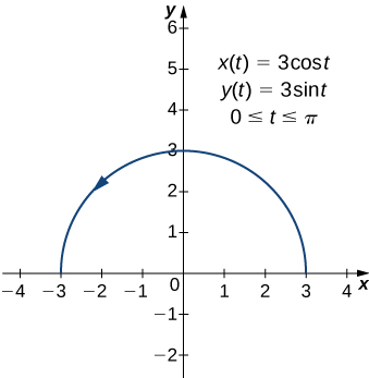
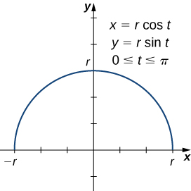
Find the arc length of the semicircle defined by the equations

Solution
The parametric curve is shown in Figure 9 below. To determine its length, we use the formula:
![\ds \begin{array}{cc}\ds \hfill s&\ds =\int\limits_{{t}_{1}}^{{t}_{2}}\sqrt{{\left(\frac{\,dx }{dt}\right)}^{2}+{\left(\frac{dy}{dt}\right)}^{2}}dt\hfill \\[5mm]\ds &\ds =\int\limits_{0}^{\pi }\sqrt{{\left(-3\phantom{\rule{0.2em}{0ex}}\text{sin}\phantom{\rule{0.2em}{0ex}}(t)\right)}^{2}+{\left(3\phantom{\rule{0.2em}{0ex}}\text{cos}\phantom{\rule{0.2em}{0ex}}(t)\right)}^{2}}dt\hfill \\[5mm]\ds &\ds =\int\limits_{0}^{\pi }\sqrt{9\phantom{\rule{0.2em}{0ex}}{\text{sin}}^{2}(t)+9\phantom{\rule{0.2em}{0ex}}{\text{cos}}^{2}(t)}\phantom{\rule{0.2em}{0ex}}dt\hfill \\[5mm]\ds &\ds =\int\limits_{0}^{\pi }\sqrt{9\left({\text{sin}}^{2}(t)+{\text{cos}}^{2}(t)\right)}dt\hfill \\[5mm]\ds &\ds =\int\limits_{0}^{\pi }3dt={3t}\Big|_{0}^{\pi }=3\pi .\hfill \end{array}](https://pressbooks.openedmb.ca/app/uploads/quicklatex/quicklatex.com-0b5c5bcf2e7f606229c9576533e11acb_l3.png "Rendered by QuickLaTeX.com")
Note that the formula for the arc length of a semicircle is  and the radius of this circle is 3. This is a great example of using calculus to derive a known geometric formula.

Find the arc length of the curve defined by the equations

Answer

We now return to the problem posed at the beginning of the section about a baseball leaving a pitcher’s hand. Ignoring the effect of air resistance (unless it is a curve ball!), the ball travels in a parabolic path. Assuming the pitcher’s hand is at the origin and the ball travels left to right in the direction of the positive x-axis, the parametric equations for this curve can be written as

where t represents time. We first calculate the distance the ball travels as a function of time. This distance is represented by the arc length. We can modify the arc length formula slightly. First rewrite the functions and using v as an independent variable, so as to eliminate any confusion with the parameter t:

Then we write the arc length formula as follows:
![\ds \begin{array}{cc}\ds \hfill s\left(t\right)&\ds =\int\limits_{0}^{t}\sqrt{{\left(\frac{\,dx }{dv}\right)}^{2}+{\left(\frac{dy}{dv}\right)}^{2}}dv\hfill \\[5mm]\ds &\ds =\int\limits_{0}^{t}\sqrt{{140}^{2}+{\left(-32v+2\right)}^{2}}dv.\hfill \end{array}](https://pressbooks.openedmb.ca/app/uploads/quicklatex/quicklatex.com-7a0ac9adafacf11e7fadf3817a6f3c30_l3.png "Rendered by QuickLaTeX.com")
The variable v acts as a dummy variable that disappears after integration, leaving the arc length as a function of time t. To integrate this expression, one needs to make a trigonometric substitution  , which will lead to a constant multiple of an integral of
  . After some technical computations, this will result in
![\ds \begin{array}{cc}\ds \hfill s\left(t\right)&\ds =-\frac{1}{32}\left[\frac{\left(-32t+2\right)}{2}\sqrt{{140}^{2}+{\left(-32t+2\right)}^{2}}+\frac{{140}^{2}}{2}\text{ln}|\left(-32t+2\right)+\sqrt{{140}^{2}+{\left(-32t+2\right)}^{2}}|\right]\hfill \\[5mm]\ds &\ds \phantom{\rule{0.6em}{0ex}}+\frac{1}{32}\left[\sqrt{{140}^{2}+{2}^{2}}+\frac{{140}^{2}}{2}\text{ln}|2+\sqrt{{140}^{2}+{2}^{2}}|\right]\hfill \\[5mm]\ds &\ds =\left(\frac{t}{2}-\frac{1}{32}\right)\sqrt{1024{t}^{2}-128t+19604}-\frac{1225}{4}\text{ln}|\left(-32t+2\right)+\sqrt{1024{t}^{2}-128t+19604}|\hfill \\[5mm]\ds &\ds \phantom{\rule{0.6em}{0ex}}+\frac{\sqrt{19604}}{32}+\frac{1225}{4}\text{ln}\left(2+\sqrt{19604}\right).\hfill \end{array}](https://pressbooks.openedmb.ca/app/uploads/quicklatex/quicklatex.com-0ca33cc90cdbc0934838f078a1d78294_l3.png "Rendered by QuickLaTeX.com")
This function represents the distance traveled by the ball as a function of time. To calculate the speed, take the derivative of this function with respect to t. While this may seem like a daunting task, it is possible to obtain the answer directly from the Fundamental Theorem of Calculus:
 Therefore,
![\ds \begin{array}{cc}\ds \hfill {s}^{\prime }\left(t\right)&\ds =\frac{d}{dt}\left[s\left(t\right)\right]\hfill \\[5mm]\ds &\ds =\frac{d}{dt}\left[\int\limits_{0}^{t}\sqrt{{140}^{2}+{\left(-32v+2\right)}^{2}}dv\right]\hfill \\[5mm]\ds &\ds =\sqrt{{140}^{2}+{\left(-32t+2\right)}^{2}}\hfill \\[5mm]\ds &\ds =\sqrt{1024{t}^{2}-128t+19604}\hfill \\[5mm]\ds &\ds =2\sqrt{256{t}^{2}-32t+4901}.\hfill \end{array}](https://pressbooks.openedmb.ca/app/uploads/quicklatex/quicklatex.com-0e2392d23ef312fd9d7075a0c0c3b65e_l3.png "Rendered by QuickLaTeX.com")
One third of a second after the ball leaves the pitcher’s hand, the distance it travels is equal to
![\ds \begin{array}{cc}\ds \hfill s\left(\frac{1}{3}\right)&\ds =\left(\frac{1\text{/}3}{2}-\frac{1}{32}\right)\sqrt{1024{\left(\frac{1}{3}\right)}^{2}-128\left(\frac{1}{3}\right)+19604}\hfill \\[5mm]\ds &\ds \phantom{\rule{0.6em}{0ex}}-\frac{1225}{4}\text{ln}|\left(-32\left(\frac{1}{3}\right)+2\right)+\sqrt{1024{\left(\frac{1}{3}\right)}^{2}-128\left(\frac{1}{3}\right)+19604}|\hfill \\[5mm]\ds &\ds \phantom{\rule{0.6em}{0ex}}+\frac{\sqrt{19604}}{32}+\frac{1225}{4}\text{ln}\left(2+\sqrt{19604}\right)\hfill \\[5mm]\ds &\ds \approx 46.69\phantom{\rule{0.2em}{0ex}}\text{feet}.\hfill \end{array}](https://pressbooks.openedmb.ca/app/uploads/quicklatex/quicklatex.com-a2d1c33796c4046ee7ac9cb0e799a4d2_l3.png "Rendered by QuickLaTeX.com")
This value is just over three quarters of the way to home plate. The speed of the ball is

This speed translates to approximately 95 mph—a major-league fastball.
Surface Area Generated by a Parametric Curve
Recall the problem of finding the surface area of a surface of revolution. In Section 2.4, we derived a formula for the surface area of a surface generated by revolving the curve  from
from  to
to  around the x-axis:

We now consider a surface of revolution generated by revolving a parametrically defined curve  around the x-axis as shown in the following figure.
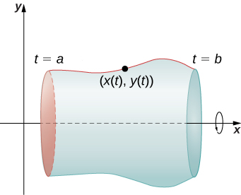
The formula for its surface area is

provided that is non-negative on
Finding Surface Area
Find the surface area of a sphere of radius r centered at the origin.
Solution
We start by parametrizing the upper semicircle with center at the origin and radius  :
:

When this curve is revolved around the x-axis, it generates a sphere of radius r. To calculate the surface area of the sphere, we use the above formula:
![\ds \begin{array}{cc}\ds \hfill S&\ds =2\pi \int\limits_{a}^{b}y\left(t\right)\sqrt{{\left({x}^{\prime }\left(t\right)\right)}^{2}+{\left({y}^{\prime }\left(t\right)\right)}^{2}}dt\hfill \\[5mm]\ds &\ds =2\pi \int\limits_{0}^{\pi }r\phantom{\rule{0.2em}{0ex}}\text{sin}\phantom{\rule{0.2em}{0ex}}(t)\sqrt{{\left( - r\phantom{\rule{0.2em}{0ex}}\text{sin}\phantom{\rule{0.2em}{0ex}}(t)\right)}^{2}+{\left(r\phantom{\rule{0.2em}{0ex}}\text{cos}\phantom{\rule{0.2em}{0ex}}(t)\right)}^{2}}dt\hfill \\[5mm]\ds &\ds =2\pi \int\limits_{0}^{\pi }r\phantom{\rule{0.2em}{0ex}}\text{sin}\phantom{\rule{0.2em}{0ex}}(t)\sqrt{{r}^{2}{\text{sin}}^{2}(t)+{r}^{2}{\text{cos}}^{2}(t)}\phantom{\rule{0.2em}{0ex}}dt\hfill \\[5mm]\ds &\ds =2\pi \int\limits_{0}^{\pi }r\phantom{\rule{0.2em}{0ex}}\text{sin}\phantom{\rule{0.2em}{0ex}}(t)\sqrt{{r}^{2}\left({\text{sin}}^{2}(t)+{\text{cos}}^{2}(t)\right)}dt\hfill \\[5mm]\ds &\ds =2\pi \int\limits_{0}^{\pi }{r}^{2}\text{sin}\phantom{\rule{0.2em}{0ex}}(t)\phantom{\rule{0.2em}{0ex}}dt\hfill \\[5mm]\ds &\ds =2\pi {r}^{2}\left({ - \text{cos}\phantom{\rule{0.2em}{0ex}}(t)}\Big|_{0}^{\pi }\right)\hfill \\[5mm]\ds &\ds =2\pi {r}^{2}\left( - \text{cos}\phantom{\rule{0.2em}{0ex}}\pi +\text{cos}\phantom{\rule{0.2em}{0ex}}0\right)\hfill \\[5mm]\ds &\ds =4\pi {r}^{2}.\hfill \end{array}](https://pressbooks.openedmb.ca/app/uploads/quicklatex/quicklatex.com-1493b1bdcb0bc94729213f320f208e0a_l3.png "Rendered by QuickLaTeX.com")
This agrees with the geometric you might have seen before.
Find the area of the surface generated by revolving the plane curve defined by the equations

around the x-axis.
Answer

Hint
When evaluating the integral, use a u-substitution.
Key Concepts
- The derivative of the parametrically defined curve and
 can be calculated using the formula
  Using the derivative, we can find the equation of a tangent line to a parametric curve.
 - If
 , the area under the parametric curve can be determined by using the formula
  where the choice of sign depends on whether is increasing or decreasing over
 ![[a,b]](https://pressbooks.openedmb.ca/app/uploads/quicklatex/quicklatex.com-2ba33d54179d658fa4d4f6a34c15cb9f_l3.png "Rendered by QuickLaTeX.com") .
. - The arc length of a parametric curve can be calculated by using the formula

- The area of a surface obtained by revolving a parametric curve around the x-axis is given by
 provided when
 ![t\in[a,b]](https://pressbooks.openedmb.ca/app/uploads/quicklatex/quicklatex.com-3c3dd904a72533b2f86965b6b5c2211b_l3.png "Rendered by QuickLaTeX.com") . If the curve is revolved around the y-axis, then the formula is
. If the curve is revolved around the y-axis, then the formula is 
provided when .
Key Equations
- Derivative of parametric equations

- Second-order derivative of parametric equations

- Area under a parametric curve
 , where the sign depends on the sign of
 - Arc length of a parametric curve

- Surface area generated by a parametric curve about a coordinate axis
 (revolving about x-axis)
 (revolving about y-axis)
Exercises
For the following exercises, find as a function of the parameter t.
1. 
Answer

2. 
3. 
Answer

4. 
For the following exercises, each set of parametric equations represents a line. Without eliminating the parameter, find the slope of each line.
5. 
Answer

6. 
7. 
Answer
0
For the following exercises, determine the slope of the tangent line at the point corresponding to the given value of the parameter.
8. 
9. 
Answer

10. 
11. 
Answer
Slope is undefined.
12. 
For the following exercises, find all points on the parametric curve where the tangent line has the given slope.
13. 
Answer
 , where
  is integer, corresponding to the points
  and
and  .
.
14. 
15. 
Answer
corresponding to the point  (note that
  is not in the domain of )
16. 
For the following exercises, write an equation of the tangent line to the given parametric curve at the point that corresponds to the specified value of the parameter t.
17. 
Answer

18. 
19. 
Answer

20. Consider the parametric curve  Find all values of the parameter that correpsond to the points on the curve where the tangent line is horizontal.
21. Consider the parametric curve 
 Find all values of the parameter that correpsond to the points on the curve where the tangent line is vertical.
Answer
 .
.
For the following exercises, find all points on the given parametric curve where the tangent line is horizontal or vertical.
22. 
23. 
Answer
No horizontal tangents. Vertical tangents at 
24. 
25. 
Answer
Horizontal tangent at  vertical tangents at
For the following exercises, find 
26. 
27. 
Answer

28. 
29. 
Answer

For the following exercises, find at the specified value of the parameter.
30. 
31. 
Answer
4
For the following exercises, find t intervals on which the given parametric curve is concave up and t intervals on which it is concave down.
32. 
33. 
Answer
Concave up on 
34. 
35. 
Answer
Concave up on  and concave down on
  .
.
36. Sketch and find the area under one arch of the cycloid  Here
Here  is a fixed real number and
  is a parameter.
37. Find the area below the curve  and above the x-axis.
Answer
2
38. Find the area enclosed by the ellipse 
39. Find the area of the region below the curve  and above the x-axis over the interval
 ![\ds \left[0,\frac{\pi }{2}\right].](https://pressbooks.openedmb.ca/app/uploads/quicklatex/quicklatex.com-df740375d205d7e1456d9478b5c1ebd8_l3.png "Rendered by QuickLaTeX.com")
Answer

For the following exercises, find the total area of the regions between the parametric curves and the x-axis. In exercises 41-43  is a fixed real number.
40. 
41.*  .
.
Answer

42.  (the “hourglass”)
43.[T]  (the “teardrop”)
Answer

For the following exercises, find the arc length of the given parametric curve.
44. 
45. 
Answer

46. 
47. 
Answer

48. 
49.  (the hypocycloid)
Answer

50. Find the length of one arch of the cycloid 
51. Find the distance traveled by a particle with position  as t varies in the given time interval:
Answer

52. Find the length of the curve 
For the following exercises, set up but do not evaluate the integral that represents the area of the surface obtained by rotating the given parametric curve about the x-axis.
53. 
Answer

54. ![\ds x=t\sin(t),\ y=\cos(2t),\ t\in\left[-\frac{\pi}4,\frac{\pi}4\right].](https://pressbooks.openedmb.ca/app/uploads/quicklatex/quicklatex.com-e520f473df8b4f1ce35de72858ef9132_l3.png "Rendered by QuickLaTeX.com")
55. ![\ds x=\sqrt{t^2+1},\ y=\frac{t+1}t,\ t\in\left[1,2\right].](https://pressbooks.openedmb.ca/app/uploads/quicklatex/quicklatex.com-201c258fd545b9b325e9e966d1918166_l3.png "Rendered by QuickLaTeX.com")
Answer

56. ![\ds x=e^t\cos(t),\ y=e^{-t}+1,\ t\in\left[-1,0\right].](https://pressbooks.openedmb.ca/app/uploads/quicklatex/quicklatex.com-7fecb8e0d23a33a6b70a52bdcdb80975_l3.png "Rendered by QuickLaTeX.com")
For the following exercises, find the area of the surface obtained by rotating the given parametric curve about the x-axis.
57. 
Answer

58. 
For the following exercises, set up but do not evaluate the integral that represents the area of the surface obtained by rotating the given parametric curve about the y-axis.
59. 
Answer

60. 
61. Find the area of the surface generated by revolving  about the y-axis.
Answer

