1.4 The Net Change Theorem and Integrals of Symmetric Functions
Learning Objectives
- Explain the significance of the net change theorem.
- Use the net change theorem to solve applied problems.
- Apply the integrals of odd and even functions.
In this section, we will reformulate the second part of the Fundamental Theorem of Calculus to obtain the Net Change Theorem that helps solving a lot of applied problems dealing with rates of change. We then discuss how symmetry of a function can simplify the integration process.
The Net Change Theorem
The net change theorem considers the integral of a rate of change. It says that when a quantity changes, the new value equals the initial value plus the integral of the rate of change of that quantity. The formula can be expressed in two ways. The second is more familiar; it is simply the Fundamental Theorem of Calculus, Part 2 written for a function  and its antiderivative
  .
.
Net Change Theorem
The new value of a changing quantity equals the initial value plus the integral of the rate of change:
![\ds \begin{array}{ll} \ds F\left(b\right)=F\left(a\right)+\int\limits_{a}^{b}F'\left(x\right)\,dx \hfill \\[5mm] \hfill \text{or}\hfill \\\ds\int\limits_{a}^{b}F'\left(x\right)\,dx =F\left(b\right)-F\left(a\right).\hfill \end{array}](https://pressbooks.openedmb.ca/app/uploads/quicklatex/quicklatex.com-757e5a015b0a8cc861a0bf330c540f62_l3.png "Rendered by QuickLaTeX.com")
Subtracting  from both sides of the first equation yields the second equation. Since they are equivalent formulas, which one we use depends on the application.
The net change theorem has a wide variety of applications. Net change can be applied to area, distance, and volume, to name only a few of them. Net change accounts for negative quantities automatically without having to write more than one integral. To illustrate, let’s apply the net change theorem to a velocity function in which the result is displacement.
We looked at a simple example of this in the Definite Integral section. Suppose a car is moving due north (the positive direction) at 40 mph between 2 p.m. and 4 p.m., then the car moves south at 30 mph between 4 p.m. and 5 p.m. We can graph this motion as illustrated below.
![A graph with the x axis marked as t and the y axis marked normally. The lines y=40 and y=-30 are drawn over [2,4] and [4,5], respectively.The areas between the lines and the x axis are shaded.](https://pressbooks.openedmb.ca/app/uploads/sites/27/2022/08/CNX_Calc_Figure_05_04_002-5.jpg)
Just as we did before, we can use definite integrals to calculate the net displacement as well as the total distance traveled. The net displacement is given by
![\ds \begin{array}{ll}\ds\int\limits_{2}^{5}v\left(t\right)dt\hfill &\ds =\int\limits_{2}^{4}40dt+\int\limits_{4}^{5}(-30)dt\hfill \\[5mm] &\ds =80-30\hfill \\[5mm] &\ds =50.\hfill \end{array}](https://pressbooks.openedmb.ca/app/uploads/quicklatex/quicklatex.com-d6d725c5b2e0e6b4d0857e440e499dac_l3.png "Rendered by QuickLaTeX.com")
Thus, at 5 p.m. the car is 50 mi north of its starting position. The total distance traveled is given by
![\ds \begin{array}{ll} \ds \int\limits_{2}^{5}|v\left(t\right)|dt\hfill &\ds =\int\limits_{2}^{4}40dt+\int\limits_{4}^{5}30dt\hfill \\[5mm] &\ds =80+30\hfill \\[5mm] &\ds =110.\hfill \end{array}](https://pressbooks.openedmb.ca/app/uploads/quicklatex/quicklatex.com-0101706edcc6841001d164cf3c1c3afb_l3.png "Rendered by QuickLaTeX.com")
Therefore, between 2 p.m. and 5 p.m., the car traveled a total of 110 mi.
To summarize, net displacement may include both positive and negative values. In other words, the velocity function accounts for both forward distance and backward distance. To find net displacement, integrate the velocity function over the interval. Total distance traveled, on the other hand, is always positive. To find the total distance traveled by an object, regardless of direction, we need to integrate the absolute value of the velocity function.
Finding Net Displacement
Given a velocity function  (in meters per second) for a particle in motion from time
  to time
  find the net displacement of the particle.
Solution
Applying the net change theorem, we have
![\ds \begin{array}{ll}\ds\int\limits_{0}^{3}\left(3t-5\right)dt\hfill &\ds =\frac{3{t}^{2}}{2}-5t{}\Big|_{0}^{3}\hfill \\[5mm]&\ds =\left[\frac{3{\left(3\right)}^{2}}{2}-5\left(3\right)\right]-0\hfill \\[5mm] &\ds =\frac{27}{2}-15\hfill \\[5mm] &\ds =\frac{27}{2}-\frac{30}{2}\hfill \\[5mm] &\ds =-\frac{3}{2}.\hfill \end{array}](https://pressbooks.openedmb.ca/app/uploads/quicklatex/quicklatex.com-c82a5ea78244fc3d522716387c4239fc_l3.png "Rendered by QuickLaTeX.com")
The net displacement is  m.
m.
![A graph of the line v(t) = 3t – 5, which goes through points (0, -5) and (5/3, 0). The area over the line and under the x axis in the interval [0, 5/3] is shaded. The area under the line and above the x axis in the interval [5/3, 3] is shaded.](https://pressbooks.openedmb.ca/app/uploads/sites/27/2022/08/CNX_Calc_Figure_05_04_003-5.jpg)
Finding the Total Distance Traveled
m/sec over a time interval ![\ds \left[0,3\right].](https://pressbooks.openedmb.ca/app/uploads/quicklatex/quicklatex.com-c8743c99f0305ee0f9b73f2ea18e5936_l3.png "Rendered by QuickLaTeX.com")
Solution
The total distance traveled includes both the positive and the negative values. Therefore, we must integrate the absolute value of the velocity function to find the total distance traveled.
To continue with the example, use two integrals to find the total distance. First, find the t-intercept of the function, since that is where the division of the interval occurs. Set the equation equal to zero and solve for t. Thus,
![\ds \begin{array}{ccc}3t-5\hfill &\ds =\hfill &\ds 0\hfill \\[3mm] \hfill 3t&\ds =\hfill &\ds 5\hfill \\[3mm] \hfill t&\ds =\hfill &\ds \frac{5}{3}.\hfill \end{array}](https://pressbooks.openedmb.ca/app/uploads/quicklatex/quicklatex.com-f48bf4d1294ac7dbd5f03cd7531583d8_l3.png "Rendered by QuickLaTeX.com")
The two subintervals are ![\ds \left[0,\frac{5}{3}\right]](https://pressbooks.openedmb.ca/app/uploads/quicklatex/quicklatex.com-d13449fcdedb3613811ba70512670671_l3.png "Rendered by QuickLaTeX.com") and
and ![\ds \left[\frac{5}{3},3\right].](https://pressbooks.openedmb.ca/app/uploads/quicklatex/quicklatex.com-64c0774bff2a1e99581d4961e1eeebaf_l3.png "Rendered by QuickLaTeX.com") To find the total distance traveled, integrate the absolute value of the function. Since the function is negative over the interval
To find the total distance traveled, integrate the absolute value of the function. Since the function is negative over the interval ![\ds \left[0,\frac{5}{3}\right],](https://pressbooks.openedmb.ca/app/uploads/quicklatex/quicklatex.com-11647fc1741e5ba833a531f60a36cebb_l3.png "Rendered by QuickLaTeX.com") we have
we have  over that interval. Over
 ![\ds \left[\frac{5}{3},3\right],](https://pressbooks.openedmb.ca/app/uploads/quicklatex/quicklatex.com-a086ce9146eeb3afcf33c7d3f1e79846_l3.png "Rendered by QuickLaTeX.com") the function is positive, so
the function is positive, so  Thus, we have
![\ds \begin{array}{ll}\ds\int\limits_{0}^{3}|v\left(t\right)|dt\hfill &\ds =\int\limits_{0}^{5\text{/}3} - v\left(t\right)dt+\int\limits_{5\text{/}3}^{3}v\left(t\right)dt\hfill \\[5mm] &\ds =\int\limits_{0}^{5\text{/}3}5-3tdt+\int\limits_{5\text{/}3}^{3}3t-5dt\hfill \\[5mm] &\ds ={\left(5t-\frac{3{t}^{2}}{2}\right)}\Big|_{0}^{5\text{/}3}+{\left(\frac{3{t}^{2}}{2}-5t\right)}\Big|_{5\text{/}3}^{3}\hfill \\[5mm] &\ds =\left[5\left(\frac{5}{3}\right)-\frac{3{\left(5\text{/}3\right)}^{2}}{2}\right]-0+\left[\frac{27}{2}-15\right]-\left[\frac{3{\left(5\text{/}3\right)}^{2}}{2}-\frac{25}{3}\right]\hfill \\[5mm] &\ds =\frac{25}{3}-\frac{25}{6}+\frac{27}{2}-15-\frac{25}{6}+\frac{25}{3}\hfill \\[5mm] &\ds =\frac{41}{6}.\hfill \end{array}](https://pressbooks.openedmb.ca/app/uploads/quicklatex/quicklatex.com-cb6df2f3df73e85d2888870afeb038f4_l3.png "Rendered by QuickLaTeX.com")
So, the total distance traveled is  m.
m.
Find the net displacement and total distance traveled in meters given the velocity function  over the interval
 ![\ds \left[0,2\right].](https://pressbooks.openedmb.ca/app/uploads/quicklatex/quicklatex.com-5b930bb4b9b14a4279911f9b0547c062_l3.png "Rendered by QuickLaTeX.com")
Answer
Net displacement:  total distance traveled:
  m
m
Hint
Note that  for
for  and
and  for
for 
Applying the Net Change Theorem
The net change theorem can be applied to the flow and consumption of fluids, as shown below.
How Many Gallons of Gasoline Are Consumed?
If the motor on a motorboat is started at and the boat consumes gasoline at the rate of  gal/hr, how much gasoline is used in the first 2 hours?
Solution
Express the problem as a definite integral, integrate, and evaluate using the Fundamental Theorem of Calculus. The limits of integration are the endpoints of the interval We have
![\ds \begin{array}{cc}\ds\int\limits_{0}^{2}\left(5-{t}^{3}\right)dt\hfill &\ds =\left(5t-\frac{{t}^{4}}{4}\right){}\Big|_{0}^{2}\hfill \\[5mm] &\ds =\left[5\left(2\right)-\frac{{\left(2\right)}^{4}}{4}\right]-0\hfill \\[5mm] &\ds =10-\frac{16}{4}\hfill \\[5mm] &\ds =6.\hfill \end{array}](https://pressbooks.openedmb.ca/app/uploads/quicklatex/quicklatex.com-98e2b12c8520b64b894a1c7b9d0dddff_l3.png "Rendered by QuickLaTeX.com")
Thus, the motorboat uses 6 gal of gas in 2 hours.
Chapter Opener: Iceboats
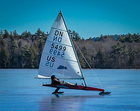
As we saw at the beginning of the chapter, top iceboat racers can attain speeds of up to five times the wind speed. Andrew is an intermediate iceboater, though, so he attains speeds equal to only twice the wind speed. Suppose Andrew takes his iceboat out one morning when a light 5-mph breeze has been blowing all morning. As Andrew gets his iceboat set up, though, the wind begins to pick up. During his first half hour of iceboating, the wind speed increases according to the function  For the second half hour of Andrew’s outing, the wind remains steady at 15 mph. In other words, the wind speed is given by
![\ds v\left(t\right)=\left\{\begin{array}{lll}20t+5\hfill &\ds \text{for}\hfill &\ds 0\le t\le \frac{1}{2}\hfill \\[2mm] 15\hfill &\ds \text{for}\hfill &\ds \frac{1}{2}\le t\le 1.\hfill \end{array}](https://pressbooks.openedmb.ca/app/uploads/quicklatex/quicklatex.com-2878709df47485992f978d9e5bc39e86_l3.png "Rendered by QuickLaTeX.com")
Recalling that Andrew’s iceboat travels at twice the wind speed, and assuming he moves in a straight line away from his starting point, how far is Andrew from his starting point after 1 hour?
Solution
To figure out how far Andrew has traveled, we need to integrate his velocity, which is twice the wind speed. Then
Distance 
Substituting the expressions we were given for  we get
![\ds \begin{array}{cc}\ds\int\limits_{0}^{1}2v\left(t\right)dt\hfill &\ds =\int\limits_{0}^{1\text{/}2}2v\left(t\right)dt+\int\limits_{1\text{/}2}^{1}2v\left(t\right)dt\hfill \\[5mm] &\ds =\int\limits_{0}^{1\text{/}2}2\left(20t+5\right)dt+\int\limits_{1\text{/}3}^{1}2\left(15\right)dt\hfill \\[5mm] &\ds =\int\limits_{0}^{1\text{/}2}\left(40t+10\right)dt+\int\limits_{1\text{/}2}^{1}30dt\hfill \\[5mm] &\ds =\left[20{t}^{2}+10t\right]{}\Big|_{0}^{1\text{/}2}+\left[30t\right]{}\Big|_{1\text{/}2}^{1}\hfill \\[5mm] &\ds =\left(\frac{20}{4}+5\right)-0+\left(30-15\right)\hfill \\[5mm] &\ds =25.\hfill \end{array}](https://pressbooks.openedmb.ca/app/uploads/quicklatex/quicklatex.com-f5089ceb9dfead4d0a4285cfc45443c9_l3.png "Rendered by QuickLaTeX.com")
So Andrew is 25 mi from his starting point after 1 hour.
Suppose that, instead of remaining steady during the second half hour of Andrew’s outing, the wind starts to die down according to the function  In other words, the wind speed is given by
![\ds v\left(t\right)=\left\{\begin{array}{lll}20t+5\hfill &\ds \text{for}\hfill &\ds 0\le t\le \frac{1}{2}\hfill \\[2mm] -10t+15\hfill &\ds \text{for}\hfill &\ds \frac{1}{2}\le t\le 1.\hfill \end{array}](https://pressbooks.openedmb.ca/app/uploads/quicklatex/quicklatex.com-f798d31d8afe163bc3ca75c13ac60e11_l3.png "Rendered by QuickLaTeX.com")
Under these conditions, how far from his starting point is Andrew after 1 hour?
Answer
17.5 mi
Hint
Don’t forget that Andrew’s iceboat moves twice as fast as the wind.
Integrating Even and Odd Functions
Definite integrals have many more applications, in particular, we will use them to calculate volumes and surface areas of solids of revolution, and lengths of the curves. It often happens that we need to integrate a function over an interval of the form ![[-a,a]](https://pressbooks.openedmb.ca/app/uploads/quicklatex/quicklatex.com-3b268037eaf4acb05d836f84db905e03_l3.png "Rendered by QuickLaTeX.com") and, in these cases, having a symmetric, that is, odd or even, integrand function can significantly simplify the computations.
and, in these cases, having a symmetric, that is, odd or even, integrand function can significantly simplify the computations.
Recall that an even function is a function satisfying  for all x in the domain—that is, the function is unchanged when x is replaced with −x. The graphs of even functions are symmetric about the y-axis. An odd function satisfies
  for all x in the domain, and the graph of such a function is symmetric about the origin.
When the limits of integration are −a and a, integrals of even functions involve two equal areas, because the graphs are symmetric about the y-axis, and integrals of odd functions evaluate to zero because the areas above and below the x-axis are equal.
Integrals of Even and Odd Functions
Suppose that the function  is continuous over the interval .
- If is even, that is,
 then
then

- If is odd, that is,
 then
then

Integrating an Even Function
Integrate the even function  and verify that the integration formula for even functions holds.
Solution
First, we formally verify that the integrand function is even. Let  . Then
  , which precisely means that is even. We then have
![\ds \begin{array}{ll}\ds\int\limits_{-2}^{2}\left(3{x}^{8}-2\right)\,dx \hfill &\ds =\left(\frac{{x}^{9}}{3}-2x\right){}\Big|_{-2}^{2}\hfill \\[5mm] &\ds =\left[\frac{{\left(2\right)}^{9}}{3}-2\left(2\right)\right]-\left[\frac{{\left(-2\right)}^{9}}{3}-2\left(-2\right)\right]\hfill \\[5mm] &\ds =\left(\frac{512}{3}-4\right)-\left(-\frac{512}{3}+4\right)\hfill \\[5mm] &\ds =\frac{1000}{3}.\hfill \end{array}](https://pressbooks.openedmb.ca/app/uploads/quicklatex/quicklatex.com-bd5a26fc34e3d95639c688f79ac3caa4_l3.png "Rendered by QuickLaTeX.com")
To verify the integration formula for even functions, we can calculate the integral from 0 to 2, then double it and check to make sure we get the same answer.
![\ds \begin{array}{ll}\ds\int\limits_{0}^{2}\left(3{x}^{8}-2\right)\,dx \hfill &\ds =\left(\frac{{x}^{9}}{3}-2x\right){}\Big|_{0}^{2}\hfill \\[5mm] &\ds =\frac{512}{3}-4\hfill \\[5mm] &\ds =\frac{500}{3}\hfill \end{array}](https://pressbooks.openedmb.ca/app/uploads/quicklatex/quicklatex.com-22a6efb0e83e74de18105666173ca004_l3.png "Rendered by QuickLaTeX.com")
Since  we have verified the formula for even functions in this particular example.
Integrating an Odd Function
Verify that the function  is odd and use this fact to evaluate the definite integral
  .
.
Solution
Substituting  into , we obtain
![\ds \begin{array}{ll}f(-x)&\ds =\sin^3(-x)((-x)^2+1)\hfill\\[5mm]&\ds =(-\sin(x))^3(x^2+1)\hfill\\[5mm]&\ds =-\sin^3(x)(x^2+1)\hfill\\[5mm]&\ds =-f(x),\end{array}](https://pressbooks.openedmb.ca/app/uploads/quicklatex/quicklatex.com-91679426def62c0f81a455e6f269cae8_l3.png "Rendered by QuickLaTeX.com")
which proves that is odd. Because is continuous over the whole real line as a product of a polynomial and a sine function, it is also continuous over ![[-5,5]](https://pressbooks.openedmb.ca/app/uploads/quicklatex/quicklatex.com-30a1b3587d0ace9b555970fabae509e9_l3.png "Rendered by QuickLaTeX.com") , and we can apply the above result to conclude that
, and we can apply the above result to conclude that  .
.
Use the properties of the integrals of symmetric functions to evaluate 
Answer

Key Concepts
- The net change theorem states that when a quantity changes, the final value equals the initial value plus the integral of the rate of change. Net change can be a positive number, a negative number, or zero.
- The area under an even function over a symmetric interval can be calculated by doubling the area over the positive x-axis. For an odd function, the integral over a symmetric interval equals zero, because the areas above and below the x-axis cancel each other.
Key Equations
- Net Change Theorem
 or
or 
Exercises
1. Suppose that a particle moves along a straight line with velocity  (in meters per second), where
  . Find the displacement at time t and the total distance traveled up to
Answer
 , the total distance traveled is
2. Suppose that a particle moves along a straight line with velocity defined by  where
where  (in meters per second). Find the displacement at time t and the total distance traveled up to
3. Suppose that a particle moves along a straight line with velocity defined by  where (in meters per second). Find the total distance traveled up to
Answer
The total distance traveled is 
4. Suppose that a particle moves along a straight line with acceleration defined by  where (in meters per second). Find the velocity and displacement at time t and the total distance traveled up to
  if
if  and
and 
5. A ball is thrown upward from a height of 1.5 m at an initial speed of 40 m/sec. Acceleration resulting from gravity is −9.8 m/sec2. Neglecting air resistance, solve for the velocity  and the height
  of the ball t seconds after it is thrown and before it returns to the ground.
Answer
 m/s
m/s
6. A ball is thrown upward from a height of 3 m at an initial speed of 60 m/sec. Acceleration resulting from gravity is −9.8 m/sec2. Neglecting air resistance, solve for the velocity and the height of the ball t seconds after it is thrown and before it returns to the ground.
7. Water flows into a conical tank with volume  up to height x. If water flows into the tank at a rate of 1 m3/min, find the height of water in the tank after 5 min. Find the change in height between 5 min and 10 min.
Answer
At  the height of water is
  The net change in height from
  to
to  is
is  m.
m.
8. A horizontal cylindrical tank has cross-sectional area  at height x meters above the bottom when
- The volume V between heights a and b is
 Find the volume at heights between 2 m and 3 m.
 - Suppose that oil is being pumped into the tank at a rate of 50 L/min. Using the chain rule,
 at how many meters per minute is the height of oil in the tank changing, expressed in terms of x, when the height is at x meters?
 - How long does it take to fill the tank to 3 m starting from a fill level of 2 m?
9. The following table lists the electrical power in gigawatts—the rate at which energy is consumed—used in a certain city for different hours of the day, in a typical 24-hour period, with hour 1 corresponding to midnight to 1 a.m.
| Hour | Power | Hour | Power |
|---|---|---|---|
| 1 | 28 | 13 | 48 |
| 2 | 25 | 14 | 49 |
| 3 | 24 | 15 | 49 |
| 4 | 23 | 16 | 50 |
| 5 | 24 | 17 | 50 |
| 6 | 27 | 18 | 50 |
| 7 | 29 | 19 | 46 |
| 8 | 32 | 20 | 43 |
| 9 | 34 | 21 | 42 |
| 10 | 39 | 22 | 40 |
| 11 | 42 | 23 | 37 |
| 12 | 46 | 24 | 34 |
Find the total amount of power in gigawatt-hours (gW-h) consumed by the city in a typical 24-hour period.
Answer
The total daily power consumption is estimated as the sum of the hourly power rates, or 911 gW-h.
10. The average residential electrical power use (in hundreds of watts) per hour is given in the following table.
| Hour | Power | Hour | Power |
|---|---|---|---|
| 1 | 8 | 13 | 12 |
| 2 | 6 | 14 | 13 |
| 3 | 5 | 15 | 14 |
| 4 | 4 | 16 | 15 |
| 5 | 5 | 17 | 17 |
| 6 | 6 | 18 | 19 |
| 7 | 7 | 19 | 18 |
| 8 | 8 | 20 | 17 |
| 9 | 9 | 21 | 16 |
| 10 | 10 | 22 | 16 |
| 11 | 10 | 23 | 13 |
| 12 | 11 | 24 | 11 |
- Compute the average total energy used in a day in kilowatt-hours (kWh).
- If a ton of coal generates 1842 kWh, how long does it take for an average residence to burn a ton of coal?
- Explain why the data might fit a plot of the form

11. The data in the following table are used to estimate the average power output produced by Peter Sagan for each of the last 18 sec of Stage 1 of the 2012 Tour de France.
| Second | Watts | Second | Watts |
|---|---|---|---|
| 1 | 600 | 10 | 1200 |
| 2 | 500 | 11 | 1170 |
| 3 | 575 | 12 | 1125 |
| 4 | 1050 | 13 | 1100 |
| 5 | 925 | 14 | 1075 |
| 6 | 950 | 15 | 1000 |
| 7 | 1050 | 16 | 950 |
| 8 | 950 | 17 | 900 |
| 9 | 1100 | 18 | 780 |
Estimate the net energy used in kilojoules (kJ), noting that 1W = 1 J/s, and the average power output by Sagan during this time interval.
Answer
17 kJ
12. The data in the following table are used to estimate the average power output produced by Peter Sagan for each 15-min interval of Stage 1 of the 2012 Tour de France.
| Minutes | Watts | Minutes | Watts |
|---|---|---|---|
| 15 | 200 | 165 | 170 |
| 30 | 180 | 180 | 220 |
| 45 | 190 | 195 | 140 |
| 60 | 230 | 210 | 225 |
| 75 | 240 | 225 | 170 |
| 90 | 210 | 240 | 210 |
| 105 | 210 | 255 | 200 |
| 120 | 220 | 270 | 220 |
| 135 | 210 | 285 | 250 |
| 150 | 150 | 300 | 400 |
Estimate the net energy used in kilojoules, noting that 1W = 1 J/s.
13. The distribution of incomes as of 2012 in the United States in $5000 increments is given in the following table. The kth row denotes the percentage of households with incomes between  and
and  The row
  contains all households with income between $200,000 and $250,000 and
  accounts for all households with income exceeding $250,000.
| 0 | 3.5 | 21 | 1.5 |
| 1 | 4.1 | 22 | 1.4 |
| 2 | 5.9 | 23 | 1.3 |
| 3 | 5.7 | 24 | 1.3 |
| 4 | 5.9 | 25 | 1.1 |
| 5 | 5.4 | 26 | 1.0 |
| 6 | 5.5 | 27 | 0.75 |
| 7 | 5.1 | 28 | 0.8 |
| 8 | 4.8 | 29 | 1.0 |
| 9 | 4.1 | 30 | 0.6 |
| 10 | 4.3 | 31 | 0.6 |
| 11 | 3.5 | 32 | 0.5 |
| 12 | 3.7 | 33 | 0.5 |
| 13 | 3.2 | 34 | 0.4 |
| 14 | 3.0 | 35 | 0.3 |
| 15 | 2.8 | 36 | 0.3 |
| 16 | 2.5 | 37 | 0.3 |
| 17 | 2.2 | 38 | 0.2 |
| 18 | 2.2 | 39 | 1.8 |
| 19 | 1.8 | 40 | 2.3 |
| 20 | 2.1 | 41 |
- Estimate the percentage of U.S. households in 2012 with incomes less than $55,000.
- What percentage of households had incomes exceeding $85,000?
- Plot the data and try to fit its shape to that of a graph of the form
 for suitable
Answer
a. 54.3%; b. 27.00%; c. The curve in the following plot is 
14. Newton’s law of gravity states that the gravitational force exerted by an object of mass M and one of mass m with centers that are separated by a distance r is  with G an empirical constant
  The work done by a variable force over an interval
 ![\ds \left[a,b\right]](https://pressbooks.openedmb.ca/app/uploads/quicklatex/quicklatex.com-c3ac37860878a36cf1c719379b6192f8_l3.png "Rendered by QuickLaTeX.com") is defined as
is defined as  If Earth has mass
  and radius 6371 km, compute the amount of work to elevate a polar weather satellite of mass 1400 kg to its orbiting altitude of 850 km above Earth.
15. For a given motor vehicle, the maximum achievable deceleration from braking is approximately 7 m/sec2 on dry concrete. On wet asphalt, it is approximately 2.5 m/sec2. Given that 1 mph corresponds to 0.447 m/sec, find the total distance that a car travels in meters on dry concrete after the brakes are applied until it comes to a complete stop if the initial velocity is 67 mph (30 m/sec) or if the initial braking velocity is 56 mph (25 m/sec). Find the corresponding distances if the surface is slippery wet asphalt.
Answer
In dry conditions, with initial velocity  m/s,
m/s,  and, if
  In wet conditions, if
  and
and  and if
16. John is a 25-year old man who weighs 160 lb. He burns  calories/hr while riding his bike for t hours. If an oatmeal cookie has 55 cal and John eats 4t cookies during the tth hour, how many net calories has he lost after 3 hours riding his bike?
17. Sandra is a 25-year old woman who weighs 120 lb. She burns  cal/hr while walking on her treadmill. Her caloric intake from drinking Gatorade is 100t calories during the tth hour. What is her net decrease in calories after walking for 3 hours?
Answer
225 cal
18. A motor vehicle has a maximum efficiency of 33 mpg at a cruising speed of 40 mph. The efficiency drops at a rate of 0.1 mpg/mph between 40 mph and 50 mph, and at a rate of 0.4 mpg/mph between 50 mph and 80 mph. What is the efficiency in miles per gallon if the car is cruising at 50 mph? What is the efficiency in miles per gallon if the car is cruising at 80 mph? If gasoline costs $3.50/gal, what is the cost of fuel to drive 50 mi at 40 mph, at 50 mph, and at 80 mph?
19. Although some engines are more efficient at given a horsepower than others, on average, fuel efficiency decreases with horsepower at a rate of  mpg/horsepower. If a typical 50-horsepower engine has an average fuel efficiency of 32 mpg, what is the average fuel efficiency of an engine with the following horsepower: 150, 300, 450?
Answer

20. [T] The following table lists the 2013 schedule of federal income tax versus taxable income.
| Taxable Income Range | The Tax Is … | … Of the Amount Over |
|---|---|---|
| $0–$8925 | 10% | $0 |
| $8925–$36,250 | $892.50 + 15% | $8925 |
| $36,250–$87,850 | $4,991.25 + 25% | $36,250 |
| $87,850–$183,250 | $17,891.25 + 28% | $87,850 |
| $183,250–$398,350 | $44,603.25 + 33% | $183,250 |
| $398,350–$400,000 | $115,586.25 + 35% | $398,350 |
 $400,000 $400,000 |
$116,163.75 + 39.6% | $400,000 |
Suppose that Steve just received a $10,000 raise. How much of this raise is left after federal taxes if Steve’s salary before receiving the raise was $40,000? If it was $90,000? If it was $385,000?
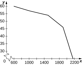
21. [T] The following table provides hypothetical data regarding the level of service for a certain highway.
| Highway Speed Range (mph) | Vehicles per Hour per Lane | Density Range (vehicles/mi) |
|---|---|---|
 |
< 600 | < 10 |
| 60–57 | 600–1000 | 10–20 |
| 57–54 | 1000–1500 | 20–30 |
| 54–46 | 1500–1900 | 30–45 |
| 46–30 | 1900–2100 | 45–70 |
| <30 | Unstable | 70–200 |
- Plot vehicles per hour per lane on the x-axis and highway speed on the y-axis.
- Compute the average decrease in speed (in miles per hour) per unit increase in congestion (vehicles per hour per lane) as the latter increases from 600 to 1000, from 1000 to 1500, and from 1500 to 2100. Does the decrease in miles per hour depend linearly on the increase in vehicles per hour per lane?
- Plot minutes per mile (60 times the reciprocal of miles per hour) as a function of vehicles per hour per lane. Is this function linear?
Answer
a.
b. Between 600 and 1000 the average decrease in vehicles per hour per lane is −0.0075. Between 1000 and 1500 it is −0.006 per vehicles per hour per lane, and between 1500 and 2100 it is −0.04 vehicles per hour per lane. c.
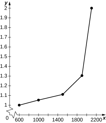
The graph is nonlinear, with minutes per mile increasing dramatically as vehicles per hour per lane reach 2000.
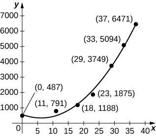
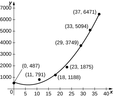
For the next two exercises use the data in the following table, which displays bald eagle populations from 1963 to 2000 in the continental United States.
| Year | Population of Breeding Pairs of Bald Eagles |
|---|---|
| 1963 | 487 |
| 1974 | 791 |
| 1981 | 1188 |
| 1986 | 1875 |
| 1992 | 3749 |
| 1996 | 5094 |
| 2000 | 6471 |
22. [T] The graph below plots the quadratic  against the data in preceding table, normalized so that corresponds to 1963. Estimate the average number of bald eagles per year present for the 37 years by computing the average value of p over
 ![\ds \left[0,37\right].](https://pressbooks.openedmb.ca/app/uploads/quicklatex/quicklatex.com-2622cd9c5b3331e40b674008abec1901_l3.png "Rendered by QuickLaTeX.com")
23. [T] The graph below plots the cubic  against the data in the preceding table, normalized so that corresponds to 1963. Estimate the average number of bald eagles per year present for the 37 years by computing the average value of p over
Answer

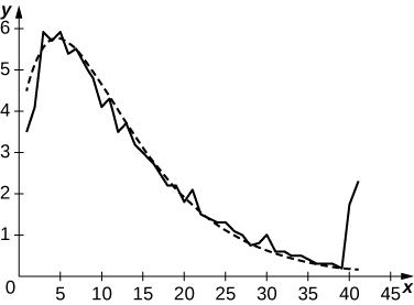
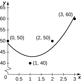
24. [T] Suppose you go on a road trip and record your speed at every half hour, as compiled in the following table. The best quadratic fit to the data is  shown in the accompanying graph. Integrate q to estimate the total distance driven over the 3 hours.
| Time (hr) | Speed (mph) |
|---|---|
| 0 (start) | 50 |
| 1 | 40 |
| 2 | 50 |
| 3 | 60 |
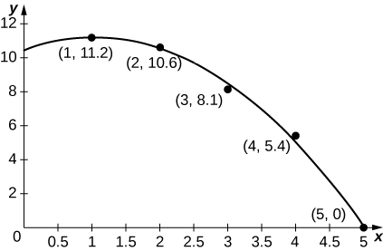
As a car accelerates, it does not accelerate at a constant rate; rather, the acceleration is variable. For the following exercises, use the following table, which contains the acceleration measured at every second as a driver merges onto a freeway.
| Time (sec) | Acceleration (mph/sec) |
|---|---|
| 1 | 11.2 |
| 2 | 10.6 |
| 3 | 8.1 |
| 4 | 5.4 |
| 5 | 0 |
25. [T] The accompanying graph plots the best quadratic fit,  to the data from the preceding table. Compute the average value of
  to estimate the average acceleration between and
Answer
Average acceleration is  mph/s
mph/s
26. [T] Using your acceleration equation from the previous exercise, find the corresponding velocity equation. Assuming the final velocity is 0 mph, find the velocity at time 
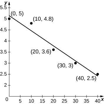
27. [T] An athlete runs by a motion detector, which records her speed, as displayed in the following table. The best linear fit to this data,  is shown in the accompanying graph. Use the average value of
  between and
  to estimate the runner’s average speed.
| Minutes | Speed (m/sec) |
|---|---|
| 0 | 5 |
| 10 | 4.8 |
| 20 | 3.6 |
| 30 | 3.0 |
| 40 | 2.5 |
Answer

In the following exercises, use symmetry to evaluate the given integrals.
28. 
29. 
Answer
 , the integrand is odd.
30. 
31. 
Answer

Glossary
- net change theorem
- if we know the rate of change of a quantity, the net change theorem says the future quantity is equal to the initial quantity plus the integral of the rate of change of the quantity
