Learning Objectives
- Analyze a function and its derivatives to draw its graph.
We have shown how to use the first and second derivatives of a function to describe the shape of a graph. Now we put everything together with other features to graph a function [latex]f[/latex].
Guidelines for Drawing the Graph of a Function
We now have enough analytical tools to draw graphs of a wide variety of algebraic and transcendental functions. Before showing how to graph specific functions, let’s look at a general strategy to use when graphing any function.
Problem-Solving Strategy: Drawing the Graph of a Function
Given a function [latex]f,[/latex] use the following steps to sketch a graph of [latex]f\text{:}[/latex]
- Determine the domain of the function.
- Locate the [latex]x[/latex]– and [latex]y[/latex]-intercepts.
- Evaluate [latex]\underset{x\to \infty }{\text{lim}}f(x)[/latex] and [latex]\underset{x\to -\infty }{\text{lim}}f(x)[/latex] to determine horizontal or oblique asymptote .
- Determine whether [latex]f[/latex] has any vertical asymptotes.
- Calculate [latex]{f}^{\prime }.[/latex] Find all critical numbers and determine the intervals where [latex]f[/latex] is increasing and where [latex]f[/latex] is decreasing. Determine whether [latex]f[/latex] has any local extrema.
- Calculate [latex]f''(x).[/latex] Determine the intervals where [latex]f[/latex] is concave up and where [latex]f[/latex] is concave down. Use this information to determine whether [latex]f[/latex] has any inflection points. The second derivative can also be used as an alternate means to determine or verify that [latex]f[/latex] has a local extremum at a critical number.
Now let’s use this strategy to graph several different functions. We start by graphing a polynomial function.
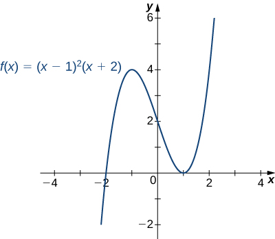
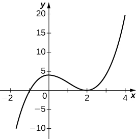
Sketching a Graph of a Polynomial
Sketch a graph of [latex]f(x)={(x-1)}^{2}(x+2).[/latex]
Solution
Step 1. Since [latex]f[/latex] is a polynomial, the domain is the set of all real numbers.
Step 2. When [latex]x=0,f(x)=2.[/latex] Therefore, the [latex]y[/latex]-intercept is [latex](0,2).[/latex] To find the [latex]x[/latex]-intercepts, we need to solve the equation [latex]{(x-1)}^{2}(x+2)=0,[/latex] gives us the [latex]x[/latex]-intercepts [latex](1,0)[/latex] and [latex](-2,0)[/latex]
Step 3. We need to evaluate the end behavior of [latex]f.[/latex] As [latex]x\to \infty ,[/latex] [latex]{(x-1)}^{2}\to \infty[/latex] and [latex](x+2)\to \infty .[/latex] Therefore, [latex]\underset{x\to \infty }{\text{lim}}f(x)=\infty .[/latex] As [latex]x\to -\infty ,[/latex] [latex]{(x-1)}^{2}\to \infty[/latex] and [latex](x+2)\to -\infty .[/latex] Therefore, [latex]\underset{x\to \infty }{\text{lim}}f(x)=-\infty .[/latex]
Step 4. Since [latex]f[/latex] is a polynomial function, it does not have any vertical asymptotes.
Step 5. The first derivative of [latex]f[/latex] is
Therefore, [latex]f[/latex] has two critical numbers: [latex]x=1,-1.[/latex] Divide the interval [latex](-\infty ,\infty )[/latex] into the three smaller intervals: [latex](-\infty ,-1),[/latex] [latex](-1,1),[/latex] and [latex](1,\infty ).[/latex] Then, choose test points [latex]x=-2,[/latex] [latex]x=0,[/latex] and [latex]x=2[/latex] from these intervals and evaluate the sign of [latex]{f}^{\prime }(x)[/latex] at each of these test points, as shown in the following table.
| Interval | Test Point | Sign of Derivative [latex]{f}^{\prime } (x)=3{x}^{2}-3=3(x-1)(x+1)[/latex] | Conclusion |
|---|---|---|---|
| [latex](-\infty ,-1)[/latex] | [latex]x=-2[/latex] | [latex](\text{+})(-)(-)=+[/latex] | [latex]f[/latex] is increasing. |
| [latex](-1,1)[/latex] | [latex]x=0[/latex] | [latex](\text{+})(-)(\text{+})=-[/latex] | [latex]f[/latex] is decreasing. |
| [latex](1,\infty )[/latex] | [latex]x=2[/latex] | [latex](\text{+})(\text{+})(\text{+})=+[/latex] | [latex]f[/latex] is increasing. |
From the table, we see that [latex]f[/latex] has a local maximum at [latex]x=-1[/latex] and a local minimum at [latex]x=1.[/latex] Evaluating [latex]f(x)[/latex] at those two points, we find that the local maximum value is [latex]f(-1)=4[/latex] and the local minimum value is [latex]f(1)=0.[/latex]
Step 6. The second derivative of [latex]f[/latex] is
The second derivative is zero at [latex]x=0.[/latex] Therefore, to determine the concavity of [latex]f,[/latex] divide the interval [latex](-\infty ,\infty )[/latex] into the smaller intervals [latex](-\infty ,0)[/latex] and [latex](0,\infty ),[/latex] and choose test points [latex]x=-1[/latex] and [latex]x=1[/latex] to determine the concavity of [latex]f[/latex] on each of these smaller intervals as shown in the following table.
| Interval | Test Point | Sign of [latex]f''(x)=6x[/latex] | Conclusion |
|---|---|---|---|
| [latex](-\infty ,0)[/latex] | [latex]x=-1[/latex] | [latex]-[/latex] | [latex]f[/latex] is concave down. |
| [latex](0,\infty )[/latex] | [latex]x=1[/latex] | [latex]+[/latex] | [latex]f[/latex] is concave up. |
We note that the information in the preceding table confirms the fact, found in step 5, that [latex]f[/latex] has a local maximum at [latex]x=-1[/latex] and a local minimum at [latex]x=1.[/latex] In addition, the information found in step 5—namely, [latex]f[/latex] has a local maximum at [latex]x=-1[/latex] and a local minimum at [latex]x=1,[/latex] and [latex]{f}^{\prime }(x)=0[/latex] at those points—combined with the fact that [latex]f''(x)[/latex] changes sign only at [latex]x=0[/latex] confirms the results found in step 6 on the concavity of [latex]f.[/latex]
Combining this information, we arrive at the graph of [latex]f(x)={(x-1)}^{2}(x+2)[/latex] shown in the following graph.
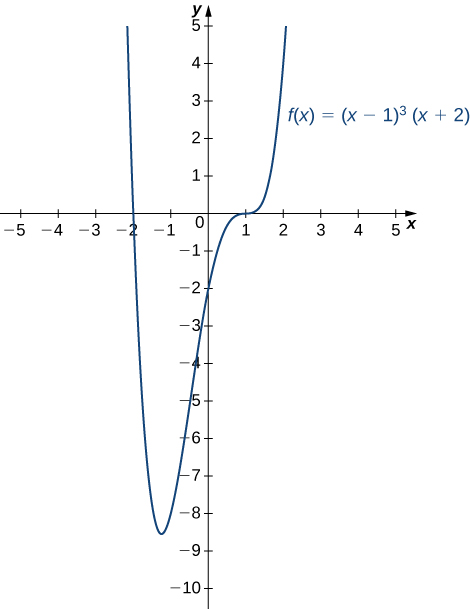
Sketch a graph of [latex]f(x)={(x-1)}^{3}(x+2).[/latex]
Solution
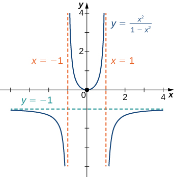
Sketching a Rational Function
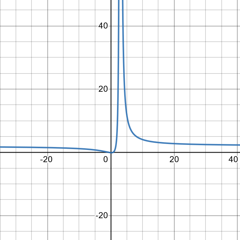
Sketch the graph of [latex]f(x)=\frac{{x}^{2}}{(1-{x}^{2})}\text{.}[/latex]
Solution
Step 1. The function [latex]f[/latex] is defined as long as the denominator is not zero. Therefore, the domain is the set of all real numbers [latex]x[/latex] except [latex]x=\pm 1.[/latex]
Step 2. Find the intercepts. If [latex]x=0,[/latex] then [latex]f(x)=0,[/latex] so 0 is an intercept. If [latex]y=0,[/latex] then [latex]\frac{{x}^{2}}{(1-{x}^{2})}=0,[/latex] which implies [latex]x=0.[/latex] Therefore, [latex](0,0)[/latex] is the only intercept.
Step 3. Evaluate the limits at infinity. Since [latex]f[/latex] is a rational function, divide the numerator and denominator by the highest power in the denominator: [latex]{x}^{2}.[/latex] We obtain
Therefore, [latex]f[/latex] has a horizontal asymptote of [latex]y=-1[/latex] as [latex]x\to \infty[/latex] and [latex]x\to -\infty .[/latex]
Step 4. To determine whether [latex]f[/latex] has any vertical asymptotes, first check to see whether the denominator has any zeroes. We find the denominator is zero when [latex]x=\pm 1.[/latex] To determine whether the lines [latex]x=1[/latex] or [latex]x=-1[/latex] are vertical asymptotes of [latex]f,[/latex] evaluate [latex]\underset{x\to 1}{\text{lim}}f(x)[/latex] and [latex]\underset{x\to -1}{\text{lim}}f(x).[/latex] By looking at each one-sided limit as [latex]x\to 1,[/latex] we see that
In addition, by looking at each one-sided limit as [latex]x\to -1,[/latex] we find that
Step 5. Calculate the first derivative:
Critical numbers occur at points [latex]x[/latex] where [latex]{f}^{\prime }(x)=0[/latex] or [latex]{f}^{\prime }(x)[/latex] is undefined. We see that [latex]{f}^{\prime }(x)=0[/latex] when [latex]x=0.[/latex] The derivative [latex]{f}^{\prime }[/latex] is not undefined at any point in the domain of [latex]f.[/latex] However, [latex]x=\pm 1[/latex] are not in the domain of [latex]f.[/latex] Therefore, to determine where [latex]f[/latex] is increasing and where [latex]f[/latex] is decreasing, divide the interval [latex](-\infty ,\infty )[/latex] into four smaller intervals: [latex](-\infty ,-1),[/latex] [latex](-1,0),[/latex] [latex](0,1),[/latex] and [latex](1,\infty ),[/latex] and choose a test point in each interval to determine the sign of [latex]{f}^{\prime }(x)[/latex] in each of these intervals. The values [latex]x=-2,[/latex] [latex]x=-\frac{1}{2},[/latex] [latex]x=\frac{1}{2},[/latex] and [latex]x=2[/latex] are good choices for test points as shown in the following table.
| Interval | Test Point | Sign of [latex]{f}^{\prime }(x)=\frac{2x}{{(1-{x}^{2})}^{2}}[/latex] | Conclusion |
|---|---|---|---|
| [latex](-\infty ,-1)[/latex] | [latex]x=-2[/latex] | [latex]-\text{/}+=-[/latex] | [latex]f[/latex] is decreasing. |
| [latex](-1,0)[/latex] | [latex]x=-1\text{/}2[/latex] | [latex]-\text{/}+=-[/latex] | [latex]f[/latex] is decreasing. |
| [latex](0,1)[/latex] | [latex]x=1\text{/}2[/latex] | [latex]+\text{/}+=+[/latex] | [latex]f[/latex] is increasing. |
| [latex](1,\infty )[/latex] | [latex]x=2[/latex] | [latex]+\text{/}+=+[/latex] | [latex]f[/latex] is increasing. |
From this analysis, we conclude that [latex]f[/latex] has a local minimum at [latex]x=0[/latex] but no local maximum.
Step 6. Calculate the second derivative:
To determine the intervals where [latex]f[/latex] is concave up and where [latex]f[/latex] is concave down, we first need to find all points [latex]x[/latex] where [latex]f''(x)=0[/latex] or [latex]f''(x)[/latex] is undefined. Since the numerator [latex]6{x}^{2}+2\ne 0[/latex] for any [latex]x,[/latex] [latex]f''(x)[/latex] is never zero. Furthermore, [latex]f''(x)[/latex] is not undefined for any [latex]x[/latex] in the domain of [latex]f.[/latex] However, as discussed earlier, [latex]x=\pm 1[/latex] are not in the domain of [latex]f.[/latex] Therefore, to determine the concavity of [latex]f,[/latex] we divide the interval [latex](-\infty ,\infty )[/latex] into the three smaller intervals [latex](-\infty ,-1),[/latex] [latex](-1,-1),[/latex] and [latex](1,\infty ),[/latex] and choose a test point in each of these intervals to evaluate the sign of [latex]f''(x).[/latex] in each of these intervals. The values [latex]x=-2,[/latex] [latex]x=0,[/latex] and [latex]x=2[/latex] are possible test points as shown in the following table.
| Interval | Test Point | Sign of [latex]f''(x)=\frac{6{x}^{2}+2}{{(1-{x}^{2})}^{3}}[/latex] | Conclusion |
|---|---|---|---|
| [latex](-\infty ,-1)[/latex] | [latex]x=-2[/latex] | [latex]+\text{/}-=-[/latex] | [latex]f[/latex] is concave down. |
| [latex](-1,-1)[/latex] | [latex]x=0[/latex] | [latex]+\text{/}+=+[/latex] | [latex]f[/latex] is concave up. |
| [latex](1,\infty )[/latex] | [latex]x=2[/latex] | [latex]+\text{/}-=-[/latex] | [latex]f[/latex] is concave down. |
Combining all this information, we arrive at the graph of [latex]f[/latex] shown below. Note that, although [latex]f[/latex] changes concavity at [latex]x=-1[/latex] and [latex]x=1,[/latex] there are no inflection points at either of these places because [latex]f[/latex] is not continuous at [latex]x=-1[/latex] or [latex]x=1.[/latex]
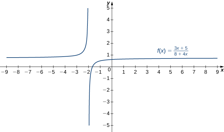
Sketch a graph of [latex]f(x)=\frac{(3x+5)}{(8+4x)}.[/latex]
Hint
A line [latex]y=L[/latex] is a horizontal asymptote of [latex]f[/latex] if the limit as [latex]x\to \infty[/latex] or the limit as [latex]x\to -\infty[/latex] of [latex]f(x)[/latex] is [latex]L.[/latex] A line [latex]x=a[/latex] is a vertical asymptote if at least one of the one-sided limits of [latex]f[/latex] as [latex]x\to a[/latex] is [latex]\infty[/latex] or [latex]-\infty .[/latex]
Solution
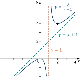
Sketching a Rational Function with an Oblique Asymptote
Sketch the graph of [latex]f(x)=\frac{{x}^{2}}{(x-1)}[/latex]
Solution
Step 1. The domain of [latex]f[/latex] is the set of all real numbers [latex]x[/latex] except [latex]x=1.[/latex]
Step 2. Find the intercepts. We can see that when [latex]x=0,[/latex] [latex]f(x)=0,[/latex] so [latex](0,0)[/latex] is the only intercept.
Step 3. Evaluate the limits at infinity. Since the degree of the numerator is one more than the degree of the denominator, [latex]f[/latex] must have an oblique asymptote. To find the oblique asymptote, use long division of polynomials to write
Since [latex]1\text{/}(x-1)\to 0[/latex] as [latex]x\to \pm \infty ,[/latex] [latex]f(x)[/latex] approaches the line [latex]y=x+1[/latex] as [latex]x\to \pm \infty .[/latex] The line [latex]y=x+1[/latex] is an oblique asymptote for [latex]f.[/latex]
Step 4. To check for vertical asymptotes, look at where the denominator is zero. Here the denominator is zero at [latex]x=1.[/latex] Looking at both one-sided limits as [latex]x\to 1,[/latex] we find
Therefore, [latex]x=1[/latex] is a vertical asymptote, and we have determined the behavior of [latex]f[/latex] as [latex]x[/latex] approaches 1 from the right and the left.
Step 5. Calculate the first derivative:
We have [latex]{f}^{\prime }(x)=0[/latex] when [latex]{x}^{2}-2x=x(x-2)=0.[/latex] Therefore, [latex]x=0[/latex] and [latex]x=2[/latex] are critical numbers. Since [latex]f[/latex] is undefined at [latex]x=1,[/latex] we need to divide the interval [latex](-\infty ,\infty )[/latex] into the smaller intervals [latex](-\infty ,0),[/latex] [latex](0,1),[/latex] [latex](1,2),[/latex] and [latex](2,\infty ),[/latex] and choose a test point from each interval to evaluate the sign of [latex]{f}^{\prime }(x)[/latex] in each of these smaller intervals. For example, let [latex]x=-1,[/latex] [latex]x=\frac{1}{2},[/latex] [latex]x=\frac{3}{2},[/latex] and [latex]x=3[/latex] be the test points as shown in the following table.
| Interval | Test Point | Sign of [latex]{f}^{\prime } (x)=\frac{{x}^{2}-2x}{{(x-1)}^{2}}=\frac{x(x-2)}{{(x-1)}^{2}}[/latex] | Conclusion |
|---|---|---|---|
| [latex](-\infty ,0)[/latex] | [latex]x=-1[/latex] | [latex](-)(-)\text{/}+=+[/latex] | [latex]f[/latex] is increasing. |
| [latex](0,1)[/latex] | [latex]x=1\text{/}2[/latex] | [latex](\text{+})(-)\text{/}+=-[/latex] | [latex]f[/latex] is decreasing. |
| [latex](1,2)[/latex] | [latex]x=3\text{/}2[/latex] | [latex](\text{+})(-)\text{/}+=-[/latex] | [latex]f[/latex] is decreasing. |
| [latex](2,\infty )[/latex] | [latex]x=3[/latex] | [latex](\text{+})(\text{+})\text{/}+=+[/latex] | [latex]f[/latex] is increasing. |
From this table, we see that [latex]f[/latex] has a local maximum at [latex]x=0[/latex] and a local minimum at [latex]x=2.[/latex] The value of [latex]f[/latex] at the local maximum is [latex]f(0)=0[/latex] and the value of [latex]f[/latex] at the local minimum is [latex]f(2)=4.[/latex] Therefore, [latex](0,0)[/latex] and [latex](2,4)[/latex] are important points on the graph.
Step 6. Calculate the second derivative:
We see that [latex]f''(x)[/latex] is never zero or undefined for [latex]x[/latex] in the domain of [latex]f.[/latex] Since [latex]f[/latex] is undefined at [latex]x=1,[/latex] to check concavity we just divide the interval [latex](-\infty ,\infty )[/latex] into the two smaller intervals [latex](-\infty ,1)[/latex] and [latex](1,\infty ),[/latex] and choose a test point from each interval to evaluate the sign of [latex]f''(x)[/latex] in each of these intervals. The values [latex]x=0[/latex] and [latex]x=2[/latex] are possible test points as shown in the following table.
| Interval | Test Point | Sign of [latex]f''(x)=\frac{2}{{(x-1)}^{3}}[/latex] | Conclusion |
|---|---|---|---|
| [latex](-\infty ,1)[/latex] | [latex]x=0[/latex] | [latex]+\text{/}-=-[/latex] | [latex]f[/latex] is concave down. |
| [latex](1,\infty )[/latex] | [latex]x=2[/latex] | [latex]+\text{/}+=+[/latex] | [latex]f[/latex] is concave up. |
From the information gathered, we arrive at the following graph for [latex]f.[/latex]
Find the oblique asymptote for [latex]f(x)=\frac{(3{x}^{3}-2x+1)}{(2{x}^{2}-4)}.[/latex]
Hint
Use long division of polynomials.
Solution
[latex]y=\frac{3}{2}x[/latex]
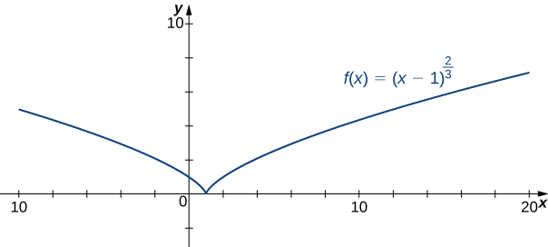
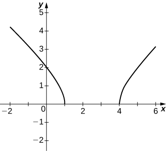
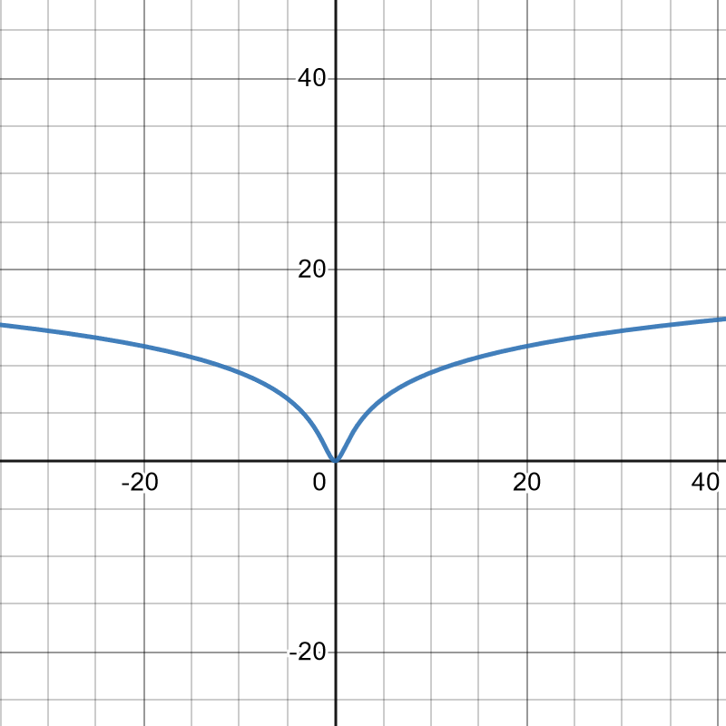
Sketching the Graph of a Function with a Cusp
Sketch a graph of [latex]f(x)={(x-1)}^{2\text{/}3}.[/latex]
Solution
Step 1. Since the cube-root function is defined for all real numbers [latex]x[/latex] and [latex]{(x-1)}^{2\text{/}3}={(\sqrt[3]{x-1})}^{2},[/latex] the domain of [latex]f[/latex] is all real numbers.
Step 2: To find the [latex]y[/latex]-intercept, evaluate [latex]f(0).[/latex] Since [latex]f(0)=1,[/latex] the [latex]y[/latex]-intercept is [latex](0,1).[/latex] To find the [latex]x[/latex]-intercept, solve [latex]{(x-1)}^{2\text{/}3}=0.[/latex] The solution of this equation is [latex]x=1,[/latex] so the [latex]x[/latex]-intercept is [latex](1,0).[/latex]
Step 3: Since [latex]\underset{x\to \pm \infty }{\text{lim}}{(x-1)}^{2\text{/}3}=\infty ,[/latex] the function continues to grow without bound as [latex]x\to \infty[/latex] and [latex]x\to -\infty .[/latex]
Step 4: The function has no vertical asymptotes.
Step 5: To determine where [latex]f[/latex] is increasing or decreasing, calculate [latex]{f}^{\prime }.[/latex] We find
This function is not zero anywhere, but it is undefined when [latex]x=1.[/latex] Therefore, the only critical number is [latex]x=1.[/latex] Divide the interval [latex](-\infty ,\infty )[/latex] into the smaller intervals [latex](-\infty ,1)[/latex] and [latex](1,\infty ),[/latex] and choose test points in each of these intervals to determine the sign of [latex]{f}^{\prime }(x)[/latex] in each of these smaller intervals. Let [latex]x=0[/latex] and [latex]x=2[/latex] be the test points as shown in the following table.
| Interval | Test Point | Sign of [latex]{f}^{\prime }(x)=\frac{2}{3{(x-1)}^{1\text{/}3}}[/latex] | Conclusion |
|---|---|---|---|
| [latex](-\infty ,1)[/latex] | [latex]x=0[/latex] | [latex]+\text{/}-=-[/latex] | [latex]f[/latex] is decreasing. |
| [latex](1,\infty )[/latex] | [latex]x=2[/latex] | [latex]+\text{/}+=+[/latex] | [latex]f[/latex] is increasing. |
We conclude that [latex]f[/latex] has a local minimum at [latex]x=1.[/latex] Evaluating [latex]f[/latex] at [latex]x=1,[/latex] we find that the value of [latex]f[/latex] at the local minimum is zero. Note that [latex]{f}^{\prime }(1)[/latex] is undefined, so to determine the behavior of the function at this critical number, we need to examine [latex]\underset{x\to 1}{\text{lim}}{f}^{\prime }(x).[/latex] Looking at the one-sided limits, we have
Therefore, [latex]f[/latex] has a cusp at [latex]x=1.[/latex]
Step 6: To determine concavity, we calculate the second derivative of [latex]f\text{:}[/latex]
We find that [latex]f''(x)[/latex] is defined for all [latex]x,[/latex] but is undefined when [latex]x=1.[/latex] Therefore, divide the interval [latex](-\infty ,\infty )[/latex] into the smaller intervals [latex](-\infty ,1)[/latex] and [latex](1,\infty ),[/latex] and choose test points to evaluate the sign of [latex]f''(x)[/latex] in each of these intervals. As we did earlier, let [latex]x=0[/latex] and [latex]x=2[/latex] be test points as shown in the following table.
| Interval | Test Point | Sign of [latex]f''(x)=\frac{-2}{9{(x-1)}^{4\text{/}3}}[/latex] | Conclusion |
|---|---|---|---|
| [latex](-\infty ,1)[/latex] | [latex]x=0[/latex] | [latex]-\text{/}+=-[/latex] | [latex]f[/latex] is concave down. |
| [latex](1,\infty )[/latex] | [latex]x=2[/latex] | [latex]-\text{/}+=-[/latex] | [latex]f[/latex] is concave down. |
From this table, we conclude that [latex]f[/latex] is concave down everywhere. Combining all of this information, we arrive at the following graph for [latex]f.[/latex]
Consider the function [latex]f(x)=5-{x}^{2\text{/}3}.[/latex] Determine the point on the graph where a cusp is located. Determine the end behavior of [latex]f.[/latex]
Hint
A function [latex]f[/latex] has a cusp at a point [latex]a[/latex] if [latex]f(a)[/latex] exists, [latex]{f}^{\prime } (a)[/latex] is undefined, one of the one-sided limits as [latex]x\to a[/latex] of [latex]{f}^{\prime } (x)[/latex] is [latex]+\infty ,[/latex] and the other one-sided limit is [latex]-\infty .[/latex]
Solution
The function [latex]f[/latex] has a cusp at [latex](0,5)[/latex] [latex]\underset{x\to {0}^{-}}{\text{lim}}{f}^{\prime }(x)=\infty ,[/latex] [latex]\underset{x\to {0}^{+}}{\text{lim}}{f}^{\prime }(x)=-\infty .[/latex] For end behavior, [latex]\underset{x\to \pm \infty }{\text{lim}}f(x)=-\infty .[/latex]
For the following exercises, sketch the function by finding the following:
- Determine the domain of the function.
- Determine the [latex]x[/latex]– and [latex]y[/latex]-intercepts.
- Determine any horizontal or vertical asymptotes.
- Determine the intervals where the function is increasing and where the function is decreasing. Determine whether the function has any local extrema.
- Determine the intervals where the function is concave up and where the function is concave down.
- Determine all inflection points (if any).
1. [latex]y=3{x}^{2}+2x+4[/latex]
2. [latex]y={x}^{3}-3{x}^{2}+4[/latex]
Solution
3. [latex]y=\frac{2x+1}{{x}^{2}+6x+5}[/latex]
4. [latex]y=\frac{{x}^{3}+4{x}^{2}+3x}{3x+9}[/latex]
Solution
5. [latex]y=\frac{{x}^{2}+x-2}{{x}^{2}-3x-4}[/latex]
6. [latex]y=\sqrt{{x}^{2}-5x+4}[/latex]
Solution
7. [latex]y=2x\sqrt{16-{x}^{2}}[/latex]
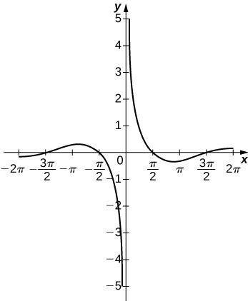
8. [latex]y=\frac{ \cos x}{x},[/latex] on [latex]x=\left[-2\pi ,2\pi \right][/latex]
Solution
9. [latex]y={e}^{x}-{x}^{3}[/latex]
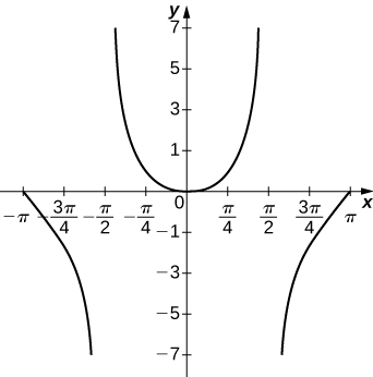
10. [latex]y=x \tan x,x=\left[-\pi ,\pi \right][/latex]
Solution
11. [latex]y=x\text{ln}(x),x < 0[/latex]
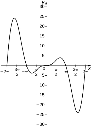
12. [latex]y={x}^{2} \sin (x),x=\left[-2\pi ,2\pi \right][/latex]
Solution
13. [latex]y = 2x + e^{-x}[/latex]
For the following exercises, sketch the graph of [latex]f[/latex] by finding the following:
- Determine the domain of the function.
- Determine the [latex]x[/latex]– and [latex]y[/latex]-intercepts.
- Determine any horizontal or vertical asymptotes.
- Determine the intervals where [latex]f[/latex] is increasing and where [latex]f[/latex] is decreasing. Determine whether [latex]f[/latex] has any local extrema.
- Determine the intervals where [latex]f[/latex] is concave up and where [latex]f[/latex] is concave down.
- Determine all inflection points (if any).
14. [latex]f(x) = \frac{2x^2 -1}{(x-3)^2}, f'(x) = \frac{-12x+2}{(x-3)^3}, f''(x) = \frac{24x+30}{(x-3)^4}[/latex]
Solution
15. [latex]f(x) = \frac{x^3}{x-4}, f'(x) = \frac{2x^3-12x}{(x-4)^2}, f''(x) = \frac{2x^3-24x^2+96x}{(x-4)^3}[/latex]
16. [latex]f(x) = 2\ln(1+x^2), f'(x) = \frac{4x}{1+x^2}, f''(x) = \frac{4(1-x^2)}{(1+x^2)^2}[/latex]
Solution
17. [latex]f(x) = \frac{e^{2x}}{x}, f'(x) = \frac{2e^{2x}-e^{2x}}{x^2}, f''(x) = \frac{2e^{2x}(2x^2-2x+1)}{x^3}[/latex]
