
Learning Objectives
- Use sigma (summation) notation to calculate sums and powers of integers.
- Use the sum of rectangular areas to approximate the area under a curve.
- Use Riemann sums to approximate area.
Archimedes was fascinated with calculating the areas of various shapes—in other words, the amount of space enclosed by the shape. He used a process that has come to be known as the method of exhaustion , which used smaller and smaller shapes, the areas of which could be calculated exactly, to fill an irregular region and thereby obtain closer and closer approximations to the total area. In this process, an area bounded by curves is filled with rectangles, triangles, and shapes with exact area formulas. These areas are then summed to approximate the area of the curved region.
In this section, we develop techniques to approximate the area between a curve, defined by a function [latex]f(x),[/latex] and the [latex]x[/latex]-axis on a closed interval [latex]\left[a,b\right].[/latex] Like Archimedes, we first approximate the area under the curve using shapes of known area (namely, rectangles). By using smaller and smaller rectangles, we get closer and closer approximations to the area. Taking a limit allows us to calculate the exact area under the curve.
Let’s start by introducing some notation to make the calculations easier. We then consider the case when [latex]f(x)[/latex] is continuous and nonnegative. Later in the chapter, we relax some of these restrictions and develop techniques that apply in more general cases.
Sigma (Summation) Notation
As mentioned, we will use shapes of known area to approximate the area of an irregular region bounded by curves. This process often requires adding up long strings of numbers. To make it easier to write down these lengthy sums, we look at some new notation here, called sigma notation (also known as summation notation). The Greek capital letter [latex]\Sigma ,[/latex] sigma, is used to express long sums of values in a compact form. For example, if we want to add all the integers from 1 to 20 without sigma notation, we have to write
We could probably skip writing a couple of terms and write
which is better, but still cumbersome. With sigma notation, we write this sum as
which is much more compact.
Typically, sigma notation is presented in the form
where [latex]{a}_{i}[/latex] describes the terms to be added, and the i is called the index . Each term is evaluated, then we sum all the values, beginning with the value when [latex]i=1[/latex] and ending with the value when [latex]i=n.[/latex] For example, an expression like [latex]\sum _{i=2}^{7}{s}_{i}[/latex] is interpreted as [latex]{s}_{2}+{s}_{3}+{s}_{4}+{s}_{5}+{s}_{6}+{s}_{7}.[/latex] Note that the index is used only to keep track of the terms to be added; it does not factor into the calculation of the sum itself. The index is therefore called a dummy variable . We can use any letter we like for the index. Typically, mathematicians use i , [latex]j[/latex], [latex]k[/latex], [latex]m[/latex], and [latex]n[/latex] for indices.
Let’s try a couple of examples of using sigma notation.
Using Sigma Notation
- Write in sigma notation and evaluate the sum of terms [latex]{3}^{i}[/latex] for [latex]i=1,2,3,4,5.[/latex]
- Write the sum in sigma notation:
[latex]1+\frac{1}{4}+\frac{1}{9}+\frac{1}{16}+\frac{1}{25}.[/latex]
Solution
- Write
[latex]\begin{array}{cc}\sum _{i=1}^{5}{3}^{i}\hfill & =3+{3}^{2}+{3}^{3}+{3}^{4}+{3}^{5}\hfill \\ & =363.\hfill \end{array}[/latex]
- The denominator of each term is a perfect square. Using sigma notation, this sum can be written as [latex]\sum _{i=1}^{5}\frac{1}{{i}^{2}}.[/latex]
Write in sigma notation and evaluate the sum of terms 2 i for [latex]i=3,4,5,6.[/latex]
Hint
Use the solving steps in (Figure) as a guide.
Solution
[latex]\sum _{i=3}^{6}{2}^{i}={2}^{3}+{2}^{4}+{2}^{5}+{2}^{6}=120[/latex]
The properties associated with the summation process are given in the following rule.
Rule: Properties of Sigma Notation
Let [latex]{a}_{1},{a}_{2}\text{,…,}{a}_{n}[/latex] and [latex]{b}_{1},{b}_{2}\text{,…,}{b}_{n}[/latex] represent two sequences of terms and let [latex]c[/latex] be a constant. The following properties hold for all positive integers [latex]n[/latex] and for integers [latex]m[/latex], with [latex]1\le m\le n.[/latex]
-
[latex]\underset{i=1}{\overset{n}{\Sigma}}c=nc[/latex]
-
[latex]\underset{i=1}{\overset{n}{\Sigma}}c{a}_{i}=c\underset{i=1}{\overset{n}{\Sigma}}{a}_{i}[/latex]
-
[latex]\underset{i=1}{\overset{n}{\Sigma}}({a}_{i}+{b}_{i})=\underset{i=1}{\overset{n}{\Sigma}}{a}_{i}+\underset{i=1}{\overset{n}{\Sigma}}{b}_{i}[/latex]
-
[latex]\underset{i=1}{\overset{n}{\Sigma}}({a}_{i}-{b}_{i})=\underset{i=1}{\overset{n}{\Sigma}}{a}_{i}-\underset{i=1}{\overset{n}{\Sigma}}{b}_{i}[/latex]
-
[latex]\underset{i=1}{\overset{n}{\Sigma}}{a}_{i}=\sum _{i=1}^{m}{a}_{i}+\sum _{i=m+1}^{n}{a}_{i}[/latex]
Proof
We prove properties 2. and 3. here, and leave proof of the other properties to the Exercises.
2. We have
3. We have
□
A few more formulas for frequently found functions simplify the summation process further. These are shown in the next rule, for sums and powers of integers, and we use them in the next set of examples.
Rule: Sums and Powers of Integers
- The sum of [latex]n[/latex] integers is given by
[latex]\underset{i=1}{\overset{n}{\Sigma}}i=1+2+\cdots+n=\frac{n(n+1)}{2}.[/latex]
- The sum of consecutive integers squared is given by
[latex]\underset{i=1}{\overset{n}{\Sigma}}{i}^{2}={1}^{2}+{2}^{2}+\cdots+{n}^{2}=\frac{n(n+1)(2n+1)}{6}.[/latex]
- The sum of consecutive integers cubed is given by
[latex]\underset{i=1}{\overset{n}{\Sigma}}{i}^{3}={1}^{3}+{2}^{3}+\cdots+{n}^{3}=\frac{{n}^{2}{(n+1)}^{2}}{4}.[/latex]
Evaluation Using Sigma Notation
Write using sigma notation and evaluate:
- The sum of the terms [latex]{(i-3)}^{2}[/latex] for [latex]i=1,2\text{,…,}200.[/latex]
- The sum of the terms [latex]({i}^{3}-{i}^{2})[/latex] for [latex]i=1,2,3,4,5,6.[/latex]
Solution
- Multiplying out [latex]{(i-3)}^{2},[/latex] we can break the expression into three terms.
[latex]\begin{array}{cc}\sum _{i=1}^{200}{(i-3)}^{2}\hfill & =\sum _{i=1}^{200}({i}^{2}-6i+9)\hfill \\ \\ \\ & =\sum _{i=1}^{200}{i}^{2}-\sum _{i=1}^{200}6i+\sum _{i=1}^{200}9\hfill \\ & =\sum _{i=1}^{200}{i}^{2}-6\sum _{i=1}^{200}i+\sum _{i=1}^{200}9\hfill \\ & =\frac{200(200+1)(400+1)}{6}-6\left[\frac{200(200+1)}{2}\right]+9(200)\hfill \\ & =2,686,700-120,600+1800\hfill \\ & =2,567,900\hfill \end{array}[/latex]
- Use sigma notation property iv. and the rules for the sum of squared terms and the sum of cubed terms.
[latex]\begin{array}{cc}\sum _{i=1}^{6}({i}^{3}-{i}^{2})\hfill & =\sum _{i=1}^{6}{i}^{3}-\sum _{i=1}^{6}{i}^{2}\hfill \\ \\ \\ \\ & =\frac{{6}^{2}{(6+1)}^{2}}{4}-\frac{6(6+1)(2(6)+1)}{6}\hfill \\ & =\frac{1764}{4}-\frac{546}{6}\hfill \\ & =350\hfill \end{array}[/latex]
Find the sum of the values of [latex]4+3i[/latex] for [latex]i=1,2\text{,…,}100.[/latex]
Hint
Use the properties of sigma notation to solve the problem.
Solution
15,550
Finding the Sum of the Function Values
Find the sum of the values of [latex]f(x)={x}^{3}[/latex] over the integers [latex]1,2,3\text{,…,}10.[/latex]
Solution
Using the formula, we have
Evaluate the sum indicated by the notation [latex]\sum _{k=1}^{20}(2k+1).[/latex]
Hint
Use the rule on sum and powers of integers.
Solution
440
Approximating Area
Now that we have the necessary notation, we return to the problem at hand: approximating the area under a curve. Let [latex]f(x)[/latex] be a continuous, nonnegative function defined on the closed interval [latex]\left[a,b\right].[/latex] We want to approximate the area A bounded by [latex]f(x)[/latex] above, the [latex]x[/latex]-axis below, the line [latex]x=a[/latex] on the left, and the line [latex]x=b[/latex] on the right ( (Figure) ).
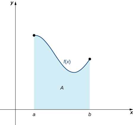
How do we approximate the area under this curve? The approach is a geometric one. By dividing a region into many small shapes that have known area formulas, we can sum these areas and obtain a reasonable estimate of the true area. We begin by dividing the interval [latex]\left[a,b\right][/latex] into [latex]n[/latex] subintervals of equal width, [latex]\frac{b-a}{n}.[/latex] We do this by selecting equally spaced points [latex]{x}_{0},{x}_{1},{x}_{2}\text{,…,}{x}_{n}[/latex] with [latex]{x}_{0}=a,{x}_{n}=b,[/latex] and
for [latex]i=1,2,3\text{,…,}n.[/latex]
We denote the width of each subinterval with the notation Δ[latex]x[/latex], so [latex]\Delta x=\frac{b-a}{n}[/latex] and
for [latex]i=1,2,3\text{,…,}n.[/latex] This notion of dividing an interval [latex]\left[a,b\right][/latex] into subintervals by selecting points from within the interval is used quite often in approximating the area under a curve, so let’s define some relevant terminology.
Definition
A set of points [latex]P=\left\{{x}_{i}\right\}[/latex] for [latex]i=0,1,2\text{,…,}n[/latex] with [latex]a={x}_{0} < {x}_{1} < {x}_{2} < \cdots < {x}_{n}=b,[/latex] which divides the interval [latex]\left[a,b\right][/latex] into subintervals of the form [latex]\left[{x}_{0},{x}_{1}\right],\left[{x}_{1},{x}_{2}\right]\text{,…,}\left[{x}_{n-1},{x}_{n}\right][/latex] is called a partition of [latex]\left[a,b\right].[/latex] If the subintervals all have the same width, the set of points forms a regular partition of the interval [latex]\left[a,b\right].[/latex]
We can use this regular partition as the basis of a method for estimating the area under the curve. We next examine two methods: the left-endpoint approximation and the right-endpoint approximation .
Rule: Left-Endpoint Approximation
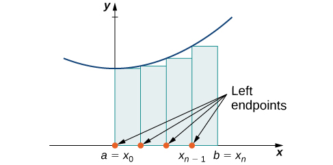
On each subinterval [latex]\left[{x}_{i-1},{x}_{i}\right][/latex] (for [latex]i=1,2,3\text{,…,}n),[/latex] construct a rectangle with width Δ[latex]x[/latex] and height equal to [latex]f({x}_{i-1}),[/latex] which is the function value at the left endpoint of the subinterval. Then the area of this rectangle is [latex]f({x}_{i-1})\Delta x.[/latex] Adding the areas of all these rectangles, we get an approximate value for A ( (Figure) ). We use the notation L n to denote that this is a left-endpoint approximation of A using [latex]n[/latex] subintervals.
The second method for approximating area under a curve is the right-endpoint approximation. It is almost the same as the left-endpoint approximation, but now the heights of the rectangles are determined by the function values at the right of each subinterval.
Rule: Right-Endpoint Approximation
Construct a rectangle on each subinterval [latex]\left[{x}_{i-1},{x}_{i}\right],[/latex] only this time the height of the rectangle is determined by the function value [latex]f({x}_{i})[/latex] at the right endpoint of the subinterval. Then, the area of each rectangle is [latex]f({x}_{i})\Delta x[/latex] and the approximation for A is given by
The notation [latex]{R}_{n}[/latex] indicates this is a right-endpoint approximation for A ( (Figure) ).

The graphs in (Figure) represent the curve [latex]f(x)=\frac{{x}^{2}}{2}.[/latex] In graph (a) we divide the region represented by the interval [latex]\left[0,3\right][/latex] into six subintervals, each of width 0.5. Thus, [latex]\Delta x=0.5.[/latex] We then form six rectangles by drawing vertical lines perpendicular to [latex]{x}_{i-1},[/latex] the left endpoint of each subinterval. We determine the height of each rectangle by calculating [latex]f({x}_{i-1})[/latex] for [latex]i=1,2,3,4,5,6.[/latex] The intervals are [latex]\left[0,0.5\right],\left[0.5,1\right],\left[1,1.5\right],\left[1.5,2\right],\left[2,2.5\right],\left[2.5,3\right].[/latex] We find the area of each rectangle by multiplying the height by the width. Then, the sum of the rectangular areas approximates the area between [latex]f(x)[/latex] and the [latex]x[/latex]-axis. When the left endpoints are used to calculate height, we have a left-endpoint approximation. Thus,
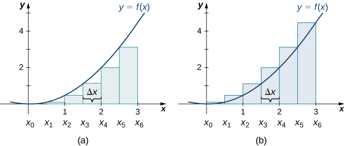
In (Figure) (b), we draw vertical lines perpendicular to [latex]{x}_{i}[/latex] such that [latex]{x}_{i}[/latex] is the right endpoint of each subinterval, and calculate [latex]f({x}_{i})[/latex] for [latex]i=1,2,3,4,5,6.[/latex] We multiply each [latex]f({x}_{i})[/latex] by Δ[latex]x[/latex] to find the rectangular areas, and then add them. This is a right-endpoint approximation of the area under [latex]f(x).[/latex] Thus,
Approximating the Area Under a Curve
Use both left-endpoint and right-endpoint approximations to approximate the area under the curve of [latex]f(x)={x}^{2}[/latex] on the interval [latex]\left[0,2\right];[/latex] use [latex]n=4.[/latex]
Solution
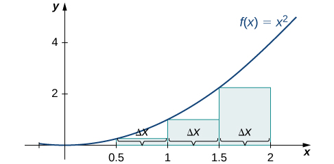
First, divide the interval [latex]\left[0,2\right][/latex] into [latex]n[/latex] equal subintervals. Using [latex]n=4,\Delta x=\frac{(2-0)}{4}=0.5.[/latex] This is the width of each rectangle. The intervals [latex]\left[0,0.5\right],\left[0.5,1\right],\left[1,1.5\right],\left[1.5,2\right][/latex] are shown in (Figure) . Using a left-endpoint approximation, the heights are [latex]f(0)=0,f(0.5)=0.25,f(1)=1,f(1.5)=2.25.[/latex] Then,
The right-endpoint approximation is shown in (Figure) . The intervals are the same, [latex]\Delta x=0.5,[/latex] but now use the right endpoint to calculate the height of the rectangles. We have
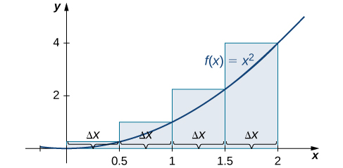
The left-endpoint approximation is 1.75; the right-endpoint approximation is 3.75.
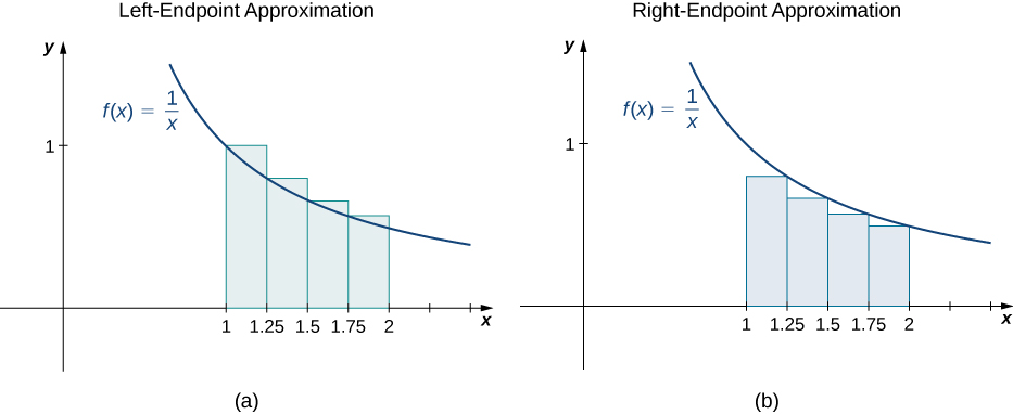
Sketch left-endpoint and right-endpoint approximations for [latex]f(x)=\frac{1}{x}[/latex] on [latex]\left[1,2\right];[/latex] use [latex]n=4.[/latex] Approximate the area using both methods.
Hint
Follow the solving strategy in (Figure) step-by-step.
Solution
The left-endpoint approximation is 0.7595. The right-endpoint approximation is 0.6345. See the below (Figure) .
Looking at (Figure) and the graphs in (Figure) , we can see that when we use a small number of intervals, neither the left-endpoint approximation nor the right-endpoint approximation is a particularly accurate estimate of the area under the curve. However, it seems logical that if we increase the number of points in our partition, our estimate of A will improve. We will have more rectangles, but each rectangle will be thinner, so we will be able to fit the rectangles to the curve more precisely.
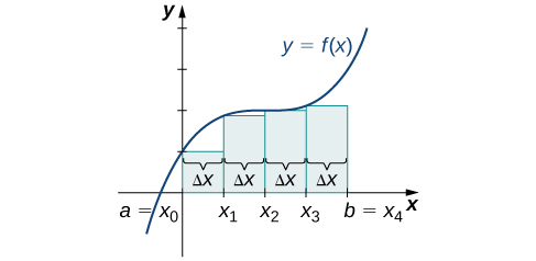
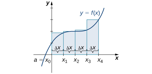
We can demonstrate the improved approximation obtained through smaller intervals with an example. Let’s explore the idea of increasing [latex]n[/latex], first in a left-endpoint approximation with four rectangles, then eight rectangles, and finally 32 rectangles. Then, let’s do the same thing in a right-endpoint approximation, using the same sets of intervals, of the same curved region. (Figure) shows the area of the region under the curve [latex]f(x)={(x-1)}^{3}+4[/latex] on the interval [latex]\left[0,2\right][/latex] using a left-endpoint approximation where [latex]n=4.[/latex] The width of each rectangle is
The area is approximated by the summed areas of the rectangles, or
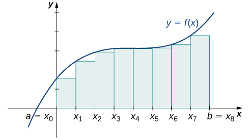
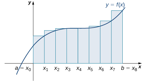
(Figure) shows the same curve divided into eight subintervals. Comparing the graph with four rectangles in (Figure) with this graph with eight rectangles, we can see there appears to be less white space under the curve when [latex]n=8.[/latex] This white space is area under the curve we are unable to include using our approximation. The area of the rectangles is
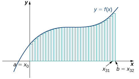
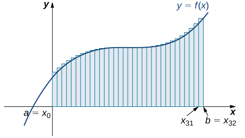
The graph in (Figure) shows the same function with 32 rectangles inscribed under the curve. There appears to be little white space left. The area occupied by the rectangles is
We can carry out a similar process for the right-endpoint approximation method. A right-endpoint approximation of the same curve, using four rectangles ( (Figure) ), yields an area
Dividing the region over the interval [latex]\left[0,2\right][/latex] into eight rectangles results in [latex]\Delta x=\frac{2-0}{8}=0.25.[/latex] The graph is shown in (Figure) . The area is
Last, the right-endpoint approximation with [latex]n=32[/latex] is close to the actual area ( (Figure) ). The area is approximately
Based on these figures and calculations, it appears we are on the right track; the rectangles appear to approximate the area under the curve better as [latex]n[/latex] gets larger. Furthermore, as [latex]n[/latex] increases, both the left-endpoint and right-endpoint approximations appear to approach an area of 8 square units. (Figure) shows a numerical comparison of the left- and right-endpoint methods. The idea that the approximations of the area under the curve get better and better as [latex]n[/latex] gets larger and larger is very important, and we now explore this idea in more detail.
| Values of [latex]n[/latex] | Approximate Area L n | Approximate Area R n |
|---|---|---|
| [latex]n=4[/latex] | 7.5 | 8.5 |
| [latex]n=8[/latex] | 7.75 | 8.25 |
| [latex]n=32[/latex] | 7.94 | 8.06 |
Forming Riemann Sums
So far we have been using rectangles to approximate the area under a curve. The heights of these rectangles have been determined by evaluating the function at either the right or left endpoints of the subinterval [latex]\left[{x}_{i-1},{x}_{i}\right].[/latex] In reality, there is no reason to restrict evaluation of the function to one of these two points only. We could evaluate the function at any point c i in the subinterval [latex]\left[{x}_{i-1},{x}_{i}\right],[/latex] and use [latex]f({x}_{i}^{*})[/latex] as the height of our rectangle. This gives us an estimate for the area of the form
A sum of this form is called a Riemann sum , named for the 19th-century mathematician Bernhard Riemann, who developed the idea.
Definition
Let [latex]f(x)[/latex] be defined on a closed interval [latex]\left[a,b\right][/latex] and let P be a regular partition of [latex]\left[a,b\right].[/latex] Let Δ[latex]x[/latex] be the width of each subinterval [latex]\left[{x}_{i-1},{x}_{i}\right][/latex] and for each i , let [latex]{x}_{i}^{*}[/latex] be any point in [latex]\left[{x}_{i-1},{x}_{i}\right].[/latex] A Riemann sum is defined for [latex]f(x)[/latex] as
Recall that with the left- and right-endpoint approximations, the estimates seem to get better and better as [latex]n[/latex] get larger and larger. The same thing happens with Riemann sums. Riemann sums give better approximations for larger values of [latex]n[/latex]. We are now ready to define the area under a curve in terms of Riemann sums.
Definition
Let [latex]f(x)[/latex] be a continuous, nonnegative function on an interval [latex]\left[a,b\right],[/latex] and let [latex]\underset{i=1}{\overset{n}{\Sigma}}f({x}_{i}^{*})\Delta x[/latex] be a Riemann sum for [latex]f(x).[/latex] Then, the area under the curve [latex]y=f(x)[/latex] on [latex]\left[a,b\right][/latex] is given by
See a graphical demonstration of the construction of a Riemann sum.
Some subtleties here are worth discussing. First, note that taking the limit of a sum is a little different from taking the limit of a function [latex]f(x)[/latex] as [latex]x[/latex] goes to infinity. Limits of sums are discussed in detail in the chapter on Sequences and Series in the second volume of this text; however, for now we can assume that the computational techniques we used to compute limits of functions can also be used to calculate limits of sums.
Second, we must consider what to do if the expression converges to different limits for different choices of [latex]\left\{{x}_{i}^{*}\right\}.[/latex] Fortunately, this does not happen. Although the proof is beyond the scope of this text, it can be shown that if [latex]f(x)[/latex] is continuous on the closed interval [latex]\left[a,b\right],[/latex] then [latex]\underset{n\to \infty }{\text{lim}}\underset{i=1}{\overset{n}{\Sigma}}f({x}_{i}^{*})\Delta x[/latex] exists and is unique (in other words, it does not depend on the choice of [latex]\left\{{x}_{i}^{*}\right\}\text{).}[/latex]
We look at some examples shortly. But, before we do, let’s take a moment and talk about some specific choices for [latex]\left\{{x}_{i}^{*}\right\}.[/latex] Although any choice for [latex]\left\{{x}_{i}^{*}\right\}[/latex] gives us an estimate of the area under the curve, we don’t necessarily know whether that estimate is too high (overestimate) or too low (underestimate). If it is important to know whether our estimate is high or low, we can select our value for [latex]\left\{{x}_{i}^{*}\right\}[/latex] to guarantee one result or the other.
If we want an overestimate, for example, we can choose [latex]\left\{{x}_{i}^{*}\right\}[/latex] such that for [latex]i=1,2,3\text{,…,}n,f({x}_{i}^{*})\ge f(x)[/latex] for all [latex]x\in \left[{x}_{i-1},{x}_{i}\right].[/latex] In other words, we choose [latex]\left\{{x}_{i}^{*}\right\}[/latex] so that for [latex]i=1,2,3\text{,…,}n,f({x}_{i}^{*})[/latex] is the maximum function value on the interval [latex]\left[{x}_{i-1},{x}_{i}\right].[/latex] If we select [latex]\left\{{x}_{i}^{*}\right\}[/latex] in this way, then the Riemann sum [latex]\underset{i=1}{\overset{n}{\Sigma}}f({x}_{i}^{*})\Delta x[/latex] is called an upper sum . Similarly, if we want an underestimate, we can choose [latex]\left\{{x}_{i}^{*}\right\}[/latex] so that for [latex]i=1,2,3\text{,…,}n,f({x}_{i}^{*})[/latex] is the minimum function value on the interval [latex]\left[{x}_{i-1},{x}_{i}\right].[/latex] In this case, the associated Riemann sum is called a lower sum . Note that if [latex]f(x)[/latex] is either increasing or decreasing throughout the interval [latex]\left[a,b\right],[/latex] then the maximum and minimum values of the function occur at the endpoints of the subintervals, so the upper and lower sums are just the same as the left- and right-endpoint approximations.
Finding Lower and Upper Sums
Find a lower sum for [latex]f(x)=10-{x}^{2}[/latex] on [latex]\left[1,2\right];[/latex] let [latex]n=4[/latex] subintervals.
With [latex]n=4[/latex] over the interval [latex]\left[1,2\right],\Delta x=\frac{1}{4}.[/latex] We can list the intervals as [latex]\left[1,1.25\right],\left[1.25,1.5\right],\left[1.5,1.75\right],\left[1.75,2\right].[/latex] Because the function is decreasing over the interval [latex]\left[1,2\right],[/latex] (Figure) shows that a lower sum is obtained by using the right endpoints.
![The graph of f(x) = 10 - x^2 from 0 to 2. It is set up for a right-end approximation of the area bounded by the curve and the x axis on [1, 2], labeled a=x0 to x4. It shows a lower sum.](https://s3-us-west-2.amazonaws.com/courses-images/wp-content/uploads/sites/2332/2018/01/11203921/CNX_Calc_Figure_05_01_014.jpg)
The Riemann sum is
The area of 7.28 is a lower sum and an underestimate.
- Find an upper sum for [latex]f(x)=10-{x}^{2}[/latex] on [latex]\left[1,2\right];[/latex] let [latex]n=4.[/latex]
- Sketch the approximation.
Hint
[latex]f(x)[/latex] is decreasing on [latex]\left[1,2\right],[/latex] so the maximum function values occur at the left endpoints of the subintervals.
Solution
- [latex]\text{Upper sum}=8.0313.[/latex]
-
![A graph of the function f(x) = 10 - x^2 from 0 to 2. It is set up for a right endpoint approximation over the area [1,2], which is labeled a=x0 to x4. It is an upper sum.](https://s3-us-west-2.amazonaws.com/courses-images/wp-content/uploads/sites/2332/2018/01/11203924/CNX_Calc_Figure_05_01_015.jpg)
Finding Lower and Upper Sums for [latex]f(x)= \sin x[/latex]
Find a lower sum for [latex]f(x)= \sin x[/latex] over the interval [latex]\left[a,b\right]=\left[0,\frac{\pi }{2}\right];[/latex] let [latex]n=6.[/latex]
Solution
Let’s first look at the graph in (Figure) to get a better idea of the area of interest.
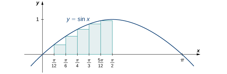
The intervals are [latex]\left[0,\frac{\pi }{12}\right],\left[\frac{\pi }{12},\frac{\pi }{6}\right],\left[\frac{\pi }{6},\frac{\pi }{4}\right],\left[\frac{\pi }{4},\frac{\pi }{3}\right],\left[\frac{\pi }{3},\frac{5\pi }{12}\right],[/latex] and [latex]\left[\frac{5\pi }{12},\frac{\pi }{2}\right].[/latex] Note that [latex]f(x)= \sin x[/latex] is increasing on the interval [latex]\left[0,\frac{\pi }{2}\right],[/latex] so a left-endpoint approximation gives us the lower sum. A left-endpoint approximation is the Riemann sum [latex]\sum _{i=0}^{5} \sin {x}_{i}(\frac{\pi }{12}).[/latex] We have
Using the function [latex]f(x)= \sin x[/latex] over the interval [latex]\left[0,\frac{\pi }{2}\right],[/latex] find an upper sum; let [latex]n=6.[/latex]
Hint
Follow the steps from (Figure) .
Solution
[latex]A\approx 1.125[/latex]
Key Concepts
- The use of sigma (summation) notation of the form [latex]\underset{i=1}{\overset{n}{\Sigma}}{a}_{i}[/latex] is useful for expressing long sums of values in compact form.
- For a continuous function defined over an interval [latex]\left[a,b\right],[/latex] the process of dividing the interval into [latex]n[/latex] equal parts, extending a rectangle to the graph of the function, calculating the areas of the series of rectangles, and then summing the areas yields an approximation of the area of that region.
- The width of each rectangle is [latex]\Delta x=\frac{b-a}{n}.[/latex]
- Riemann sums are expressions of the form [latex]\underset{i=1}{\overset{n}{\Sigma}}f({x}_{i}^{*})\Delta x,[/latex] and can be used to estimate the area under the curve [latex]y=f(x).[/latex] Left- and right-endpoint approximations are special kinds of Riemann sums where the values of [latex]\left\{{x}_{i}^{*}\right\}[/latex] are chosen to be the left or right endpoints of the subintervals, respectively.
- Riemann sums allow for much flexibility in choosing the set of points [latex]\left\{{x}_{i}^{*}\right\}[/latex] at which the function is evaluated, often with an eye to obtaining a lower sum or an upper sum.
Key Equations
- Properties of Sigma Notation
[latex]\underset{i=1}{\overset{n}{\Sigma}}c=nc[/latex]
[latex]\underset{i=1}{\overset{n}{\Sigma}}c{a}_{i}=c\underset{i=1}{\overset{n}{\Sigma}}{a}_{i}[/latex]
[latex]\underset{i=1}{\overset{n}{\Sigma}}({a}_{i}+{b}_{i})=\underset{i=1}{\overset{n}{\Sigma}}{a}_{i}+\underset{i=1}{\overset{n}{\Sigma}}{b}_{i}[/latex]
[latex]\underset{i=1}{\overset{n}{\Sigma}}({a}_{i}-{b}_{i})=\underset{i=1}{\overset{n}{\Sigma}}{a}_{i}-\underset{i=1}{\overset{n}{\Sigma}}{b}_{i}[/latex]
[latex]\underset{i=1}{\overset{n}{\Sigma}}{a}_{i}=\sum _{i=1}^{m}{a}_{i}+\sum _{i=m+1}^{n}{a}_{i}[/latex] - Sums and Powers of Integers
[latex]\underset{i=1}{\overset{n}{\Sigma}}i=1+2+\cdots+n=\frac{n(n+1)}{2}[/latex]
[latex]\underset{i=1}{\overset{n}{\Sigma}}{i}^{2}={1}^{2}+{2}^{2}+\cdots+{n}^{2}=\frac{n(n+1)(2n+1)}{6}[/latex]
[latex]\sum _{i=0}^{n}{i}^{3}={1}^{3}+{2}^{3}+\cdots+{n}^{3}=\frac{{n}^{2}{(n+1)}^{2}}{4}[/latex] - Left-Endpoint Approximation
[latex]A\approx {L}_{n}=f({x}_{0})\Delta x+f({x}_{1})\Delta x+\cdots+f({x}_{n-1})\Delta x=\underset{i=1}{\overset{n}{\Sigma}}f({x}_{i-1})\Delta x[/latex] - Right-Endpoint Approximation
[latex]A\approx {R}_{n}=f({x}_{1})\Delta x+f({x}_{2})\Delta x+\cdots+f({x}_{n})\Delta x=\underset{i=1}{\overset{n}{\Sigma}}f({x}_{i})\Delta x[/latex]
1. State whether the given sums are equal or unequal.
- [latex]\sum _{i=1}^{10}i[/latex] and [latex]\sum _{k=1}^{10}k[/latex]
- [latex]\sum _{i=1}^{10}i[/latex] and [latex]\sum _{i=6}^{15}(i-5)[/latex]
- [latex]\sum _{i=1}^{10}i(i-1)[/latex] and [latex]\sum _{j=0}^{9}(j+1)j[/latex]
- [latex]\sum _{i=1}^{10}i(i-1)[/latex] and [latex]\sum _{k=1}^{10}({k}^{2}-k)[/latex]
Solution
a. They are equal; both represent the sum of the first 10 whole numbers. b. They are equal; both represent the sum of the first 10 whole numbers. c. They are equal by substituting [latex]j=i-1.[/latex] d. They are equal; the first sum factors the terms of the second.
In the following exercises, use the rules for sums of powers of integers to compute the sums.
2. [latex]\sum _{i=5}^{10}i[/latex]
3. [latex]\sum _{i=5}^{10}{i}^{2}[/latex]
Solution
[latex]385-30=355[/latex]
Suppose that [latex]\sum _{i=1}^{100}{a}_{i}=15[/latex] and [latex]\sum _{i=1}^{100}{b}_{i}=-12.[/latex] In the following exercises, compute the sums.
4. [latex]\sum _{i=1}^{100}({a}_{i}+{b}_{i})[/latex]
5. [latex]\sum _{i=1}^{100}({a}_{i}-{b}_{i})[/latex]
Solution
[latex]15-(-12)=27[/latex]
6. [latex]\sum _{i=1}^{100}(3{a}_{i}-4{b}_{i})[/latex]
7. [latex]\sum _{i=1}^{100}(5{a}_{i}+4{b}_{i})[/latex]
Solution
[latex]5(15)+4(-12)=27[/latex]
In the following exercises, use summation properties and formulas to rewrite and evaluate the sums.
8. [latex]\sum _{k=1}^{20}100({k}^{2}-5k+1)[/latex]
9. [latex]\sum _{j=1}^{50}({j}^{2}-2j)[/latex]
Solution
[latex]\sum _{j=1}^{50}{j}^{2}-2\sum _{j=1}^{50}j=\frac{(50)(51)(101)}{6}-\frac{2(50)(51)}{2}=40,\text{}375[/latex]
10. [latex]\sum _{j=11}^{20}({j}^{2}-10j)[/latex]
11. [latex]\sum _{k=1}^{25}\left[{(2k)}^{2}-100k\right][/latex]
Solution
[latex]4\sum _{k=1}^{25}{k}^{2}-100\sum _{k=1}^{25}k=\frac{4(25)(26)(51)}{9}-50(25)(26)=-10,\text{}400[/latex]
Let [latex]{L}_{n}[/latex] denote the left-endpoint sum using [latex]n[/latex] subintervals and let [latex]{R}_{n}[/latex] denote the corresponding right-endpoint sum. In the following exercises, compute the indicated left and right sums for the given functions on the indicated interval.
12 . L 4 for [latex]f(x)=\frac{1}{x-1}[/latex] on [latex]\left[2,3\right][/latex]
13. R 4 for [latex]g(x)= \cos (\pi x)[/latex] on [latex]\left[0,1\right][/latex]
Solution
[latex]{R}_{4}=0.25[/latex]
14. L 6 for [latex]f(x)=\frac{1}{x(x-1)}[/latex] on [latex]\left[2,5\right][/latex]
15. R 6 for [latex]f(x)=\frac{1}{x(x-1)}[/latex] on [latex]\left[2,5\right][/latex]
Solution
[latex]{R}_{6}=0.372[/latex]
16. R 4 for [latex]\frac{1}{{x}^{2}+1}[/latex] on [latex]\left[-2,2\right][/latex]
17. L 4 for [latex]\frac{1}{{x}^{2}+1}[/latex] on [latex]\left[-2,2\right][/latex]
Solution
[latex]{L}_{4}=2.20[/latex]
18. R 4 for [latex]{x}^{2}-2x+1[/latex] on [latex]\left[0,2\right][/latex]
19. L 8 for [latex]{x}^{2}-2x+1[/latex] on [latex]\left[0,2\right][/latex]
Solution
[latex]{L}_{8}=0.6875[/latex]
20. Compute the left and right Riemann sums— L 4 and R 4 , respectively—for [latex]f(x)=(2-|x|)[/latex] on [latex]\left[-2,2\right].[/latex] Compute their average value and compare it with the area under the graph of [latex]f[/latex].
21. Compute the left and right Riemann sums— L 6 and R 6 , respectively—for [latex]f(x)=(3-|3-x|)[/latex] on [latex]\left[0,6\right].[/latex] Compute their average value and compare it with the area under the graph of [latex]f[/latex].
Solution
[latex]{L}_{6}=9.000={R}_{6}.[/latex] The graph of [latex]f[/latex] is a triangle with area 9.
22. Compute the left and right Riemann sums— L 4 and R 4 , respectively—for [latex]f(x)=\sqrt{4-{x}^{2}}[/latex] on [latex]\left[-2,2\right][/latex] and compare their values.
23. Compute the left and right Riemann sums— L 6 and R 6 , respectively—for [latex]f(x)=\sqrt{9-{(x-3)}^{2}}[/latex] on [latex]\left[0,6\right][/latex] and compare their values.
Solution
[latex]{L}_{6}=13.12899={R}_{6}.[/latex] They are equal.
Express the following endpoint sums in sigma notation but do not evaluate them.
24. L 30 for [latex]f(x)={x}^{2}[/latex] on [latex]\left[1,2\right][/latex]
25. L 10 for [latex]f(x)=\sqrt{4-{x}^{2}}[/latex] on [latex]\left[-2,2\right][/latex]
Solution
[latex]{L}_{10}=\frac{4}{10}\sum _{i=1}^{10}\sqrt{4-(-2+4\frac{(i-1)}{10})}[/latex]
26. R 20 for [latex]f(x)= \sin x[/latex] on [latex]\left[0,\pi \right][/latex]
27. R 100 for [latex]\text{ln}x[/latex] on [latex]\left[1,e\right][/latex]
Solution
[latex]{R}_{100}=\frac{e-1}{100}\sum _{i=1}^{100}\text{ln}(1+(e-1)\frac{i}{100})[/latex]
In the following exercises, graph the function then use a calculator or a computer program to evaluate the following left and right endpoint sums. Is the area under the curve between the left and right endpoint sums?
28. [T] L 100 and R 100 for [latex]y={x}^{2}-3x+1[/latex] on the interval [latex]\left[-1,1\right][/latex]
29. [T] L 100 and R 100 for [latex]y={x}^{2}[/latex] on the interval [latex]\left[0,1\right][/latex]
Solution
![A graph of the given function on the interval [0, 1]. It is set up for a left endpoint approximation and is an underestimate because the function is increasing. Ten rectangles are shown for visual clarity, but this behavior persists for more rectangles.](https://s3-us-west-2.amazonaws.com/courses-images/wp-content/uploads/sites/2332/2018/01/11203930/CNX_Calc_Figure_05_01_207.jpg)
[latex]{R}_{100}=0.33835,{L}_{100}=0.32835.[/latex] The plot shows that the left Riemann sum is an underestimate because the function is increasing. Similarly, the right Riemann sum is an overestimate. The area lies between the left and right Riemann sums. Ten rectangles are shown for visual clarity. This behavior persists for more rectangles.
30. [T] L 50 and R 50 for [latex]y=\frac{x+1}{{x}^{2}-1}[/latex] on the interval [latex]\left[2,4\right][/latex]
31. [T] L 100 and R 100 for [latex]y={x}^{3}[/latex] on the interval [latex]\left[-1,1\right][/latex]
Solution
![A graph of the given function over [-1,1] set up for a left endpoint approximation. It is an underestimate since the function is increasing. Ten rectangles are shown for visual clarity, but this behavior persists for more rectangles.](https://s3-us-west-2.amazonaws.com/courses-images/wp-content/uploads/sites/2332/2018/01/11203933/CNX_Calc_Figure_05_01_209.jpg)
[latex]{L}_{100}=-0.02,{R}_{100}=0.02.[/latex] The left endpoint sum is an underestimate because the function is increasing. Similarly, a right endpoint approximation is an overestimate. The area lies between the left and right endpoint estimates.
32. [T] L 50 and R 50 for [latex]y= \tan (x)[/latex] on the interval [latex]\left[0,\frac{\pi }{4}\right][/latex]
33. [T] L 100 and R 100 for [latex]y={e}^{2x}[/latex] on the interval [latex]\left[-1,1\right][/latex]
Solution
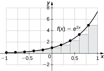
[latex]{L}_{100}=3.555,{R}_{100}=3.670.[/latex] The plot shows that the left Riemann sum is an underestimate because the function is increasing. Ten rectangles are shown for visual clarity. This behavior persists for more rectangles.
34. Let t j denote the time that it took Tejay van Garteren to ride the [latex]j[/latex]th stage of the Tour de France in 2014. If there were a total of 21 stages, interpret [latex]\sum _{j=1}^{21}{t}_{j}.[/latex]
35. Let [latex]{r}_{j}[/latex] denote the total rainfall in Portland on the [latex]j[/latex]th day of the year in 2009. Interpret [latex]\sum _{j=1}^{31}{r}_{j}.[/latex]
Solution
The sum represents the cumulative rainfall in January 2009.
36. Let [latex]{d}_{j}[/latex] denote the hours of daylight and [latex]{\delta }_{j}[/latex] denote the increase in the hours of daylight from day [latex]j-1[/latex] to day [latex]j[/latex] in Fargo, North Dakota, on the [latex]j[/latex]th day of the year. Interpret [latex]{d}_{1}+\sum _{j=2}^{365}{\delta }_{j}.[/latex]
37. To help get in shape, Joe gets a new pair of running shoes. If Joe runs 1 mi each day in week 1 and adds [latex]\frac{1}{10}[/latex] mi to his daily routine each week, what is the total mileage on Joe’s shoes after 25 weeks?
Solution
The total mileage is [latex]7×\sum _{i=1}^{25}(1+\frac{(i-1)}{10})=7×25+\frac{7}{10}×12×25=385\text{mi}.[/latex]
38. The following table gives approximate values of the average annual atmospheric rate of increase in carbon dioxide (CO 2 ) each decade since 1960, in parts per million (ppm). Estimate the total increase in atmospheric CO 2 between 1964 and 2013.
| Decade | Ppm/y |
|---|---|
| 1964–1973 | 1.07 |
| 1974–1983 | 1.34 |
| 1984–1993 | 1.40 |
| 1994–2003 | 1.87 |
| 2004–2013 | 2.07 |
39. The following table gives the approximate increase in sea level in inches over 20 years starting in the given year. Estimate the net change in mean sea level from 1870 to 2010.
| Starting Year | 20-Year Change |
|---|---|
| 1870 | 0.3 |
| 1890 | 1.5 |
| 1910 | 0.2 |
| 1930 | 2.8 |
| 1950 | 0.7 |
| 1970 | 1.1 |
| 1990 | 1.5 |
Solution
Add the numbers to get 8.1-in. net increase.
40. The following table gives the approximate increase in dollars in the average price of a gallon of gas per decade since 1950. If the average price of a gallon of gas in 2010 was $2.60, what was the average price of a gallon of gas in 1950?
| Starting Year | 10-Year Change |
|---|---|
| 1950 | 0.03 |
| 1960 | 0.05 |
| 1970 | 0.86 |
| 1980 | -0.03 |
| 1990 | 0.29 |
| 2000 | 1.12 |
41. The following table gives the percent growth of the U.S. population beginning in July of the year indicated. If the U.S. population was 281,421,906 in July 2000, estimate the U.S. population in July 2010.
| Year | % Change/Year |
|---|---|
| 2000 | 1.12 |
| 2001 | 0.99 |
| 2002 | 0.93 |
| 2003 | 0.86 |
| 2004 | 0.93 |
| 2005 | 0.93 |
| 2006 | 0.97 |
| 2007 | 0.96 |
| 2008 | 0.95 |
| 2009 | 0.88 |
( Hint: To obtain the population in July 2001, multiply the population in July 2000 by 1.0112 to get 284,573,831.)
Solution
309,389,957
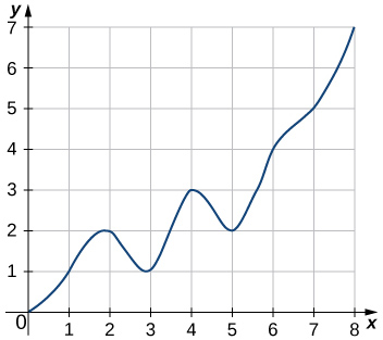
In the following exercises, estimate the areas under the curves by computing the left Riemann sums, L 8 .
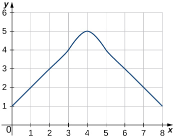
Solution
[latex]{L}_{8}=3+2+1+2+3+4+5+4=24[/latex]
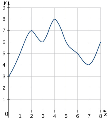
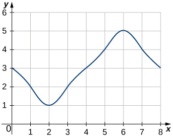
Solution
[latex]{L}_{8}=3+5+7+6+8+6+5+4=44[/latex]
46. [T] Use a computer algebra system to compute the Riemann sum, [latex]{L}_{N},[/latex] for [latex]N=10,30,50[/latex] for [latex]f(x)=\sqrt{1-{x}^{2}}[/latex] on [latex]\left[-1,1\right].[/latex]
47. [T] Use a computer algebra system to compute the Riemann sum, L N , for [latex]N=10,30,50[/latex] for [latex]f(x)=\frac{1}{\sqrt{1+{x}^{2}}}[/latex] on [latex]\left[-1,1\right].[/latex]
Solution
[latex]{L}_{10}\approx 1.7604,{L}_{30}\approx 1.7625,{L}_{50}\approx 1.76265[/latex]
48. [T] Use a computer algebra system to compute the Riemann sum, L N , for [latex]N=10,30,50[/latex] for [latex]f(x)={ \sin }^{2}x[/latex] on [latex]\left[0,2\pi \right].[/latex] Compare these estimates with π .
In the following exercises, use a calculator or a computer program to evaluate the endpoint sums R N and L N for [latex]N=1,10,100.[/latex] How do these estimates compare with the exact answers, which you can find via geometry?
49. [T] [latex]y= \cos (\pi x)[/latex] on the interval [latex]\left[0,1\right][/latex]
Solution
[latex]{R}_{1}=-1,{L}_{1}=1,{R}_{10}=-0.1,{L}_{10}=0.1,{L}_{100}=0.01,[/latex] and [latex]{R}_{100}=-0.1.[/latex] By symmetry of the graph, the exact area is zero.
50. [T] [latex]y=3x+2[/latex] on the interval [latex]\left[3,5\right][/latex]
In the following exercises, use a calculator or a computer program to evaluate the endpoint sums R N and L N for [latex]N=1,10,100.[/latex]
51. [T] [latex]y={x}^{4}-5{x}^{2}+4[/latex] on the interval [latex]\left[-2,2\right],[/latex] which has an exact area of [latex]\frac{32}{15}[/latex]
Solution
[latex]{R}_{1}=0,{L}_{1}=0,{R}_{10}=2.4499,{L}_{10}=2.4499,{R}_{100}=2.1365,{L}_{100}=2.1365[/latex]
52. [T] [latex]y=\text{ln}x[/latex] on the interval [latex]\left[1,2\right],[/latex] which has an exact area of [latex]2\text{ln}(2)-1[/latex]
53. Explain why, if [latex]f(a)\ge 0[/latex] and [latex]f[/latex] is increasing on [latex]\left[a,b\right],[/latex] that the left endpoint estimate is a lower bound for the area below the graph of [latex]f[/latex] on [latex]\left[a,b\right].[/latex]
Solution
If [latex]\left[c,d\right][/latex] is a subinterval of [latex]\left[a,b\right][/latex] under one of the left-endpoint sum rectangles, then the area of the rectangle contributing to the left-endpoint estimate is [latex]f(c)(d-c).[/latex] But, [latex]f(c)\le f(x)[/latex] for [latex]c\le x\le d,[/latex] so the area under the graph of [latex]f[/latex] between [latex]c[/latex] and [latex]d[/latex] is [latex]f(c)(d-c)[/latex] plus the area below the graph of [latex]f[/latex] but above the horizontal line segment at height [latex]f(c),[/latex] which is positive. As this is true for each left-endpoint sum interval, it follows that the left Riemann sum is less than or equal to the area below the graph of [latex]f[/latex] on [latex]\left[a,b\right].[/latex]
54. Explain why, if [latex]f(b)\ge 0[/latex] and [latex]f[/latex] is decreasing on [latex]\left[a,b\right],[/latex] that the left endpoint estimate is an upper bound for the area below the graph of [latex]f[/latex] on [latex]\left[a,b\right].[/latex]
55. Show that, in general, [latex]{R}_{N}-{L}_{N}=(b-a)×\frac{f(b)-f(a)}{N}.[/latex]
Solution
[latex]{L}_{N}=\frac{b-a}{N}\underset{i=1}{\overset{n}{\Sigma}}f(a+(b-a)\frac{i-1}{N})=\frac{b-a}{N}\sum _{i=0}^{N-1}f(a+(b-a)\frac{i}{N})[/latex] and [latex]{R}_{N}=\frac{b-a}{N}\underset{i=1}{\overset{n}{\Sigma}}f(a+(b-a)\frac{i}{N}).[/latex] The left sum has a term corresponding to [latex]i=0[/latex] and the right sum has a term corresponding to [latex]i=N.[/latex] In [latex]{R}_{N}-{L}_{N},[/latex] any term corresponding to [latex]i=1,2\text{,…,}N-1[/latex] occurs once with a plus sign and once with a minus sign, so each such term cancels and one is left with [latex]{R}_{N}-{L}_{N}=\frac{b-a}{N}(f(a+(b-a))\frac{N}{N})-(f(a)+(b-a)\frac{0}{N})=\frac{b-a}{N}(f(b)-f(a)).[/latex]
56. Explain why, if [latex]f[/latex] is increasing on [latex]\left[a,b\right],[/latex] the error between either L N or R N and the area A below the graph of [latex]f[/latex] is at most [latex](b-a)\frac{f(b)-f(a)}{N}.[/latex]
57. For each of the three graphs:
- Obtain a lower bound [latex]L(A)[/latex] for the area enclosed by the curve by adding the areas of the squares enclosed completely by the curve.
- Obtain an upper bound [latex]U(A)[/latex] for the area by adding to [latex]L(A)[/latex] the areas [latex]B(A)[/latex] of the squares enclosed partially by the curve.
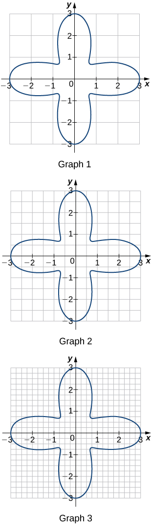
Solution
Graph 1: a. [latex]L(A)=0,B(A)=20;[/latex] b. [latex]U(A)=20.[/latex] Graph 2: a. [latex]L(A)=9;[/latex] b. [latex]B(A)=11,U(A)=20.[/latex] Graph 3: a. [latex]L(A)=11.0;[/latex] b. [latex]B(A)=4.5,U(A)=15.5.[/latex]
58. In the previous exercise, explain why [latex]L(A)[/latex] gets no smaller while [latex]U(A)[/latex] gets no larger as the squares are subdivided into four boxes of equal area.
59. A unit circle is made up of [latex]n[/latex] wedges equivalent to the inner wedge in the figure. The base of the inner triangle is 1 unit and its height is [latex]\sin (\frac{\pi }{n}).[/latex] The base of the outer triangle is [latex]B= \cos (\frac{\pi }{n})+ \sin (\frac{\pi }{n}) \tan (\frac{\pi }{n})[/latex] and the height is [latex]H=B \sin (\frac{2\pi }{n}).[/latex] Use this information to argue that the area of a unit circle is equal to π .
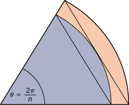
Solution
Let A be the area of the unit circle. The circle encloses [latex]n[/latex] congruent triangles each of area [latex]\frac{ \sin (\frac{2\pi }{n})}{2},[/latex] so [latex]\frac{n}{2} \sin (\frac{2\pi }{n})\le A.[/latex] Similarly, the circle is contained inside [latex]n[/latex] congruent triangles each of area [latex]\frac{BH}{2}=\frac{1}{2}( \cos (\frac{\pi }{n})+ \sin (\frac{\pi }{n}) \tan (\frac{\pi }{n})) \sin (\frac{2\pi }{n}),[/latex] so [latex]A\le \frac{n}{2} \sin (\frac{2\pi }{n})( \cos (\frac{\pi }{n}))+ \sin (\frac{\pi }{n}) \tan (\frac{\pi }{n}).[/latex] As [latex]n\to \infty ,\frac{n}{2} \sin (\frac{2\pi }{n})=\frac{\pi \sin (\frac{2\pi }{n})}{(\frac{2\pi }{n})}\to \pi ,[/latex] so we conclude [latex]\pi \le A.[/latex] Also, as [latex]n\to \infty , \cos (\frac{\pi }{n})+ \sin (\frac{\pi }{n}) \tan (\frac{\pi }{n})\to 1,[/latex] so we also have [latex]A\le \pi .[/latex] By the squeeze theorem for limits, we conclude that [latex]A=\pi .[/latex]
Glossary
- left-endpoint approximation
- an approximation of the area under a curve computed by using the left endpoint of each subinterval to calculate the height of the vertical sides of each rectangle
- lower sum
- a sum obtained by using the minimum value of [latex]f(x)[/latex] on each subinterval
- partition
- a set of points that divides an interval into subintervals
- regular partition
- a partition in which the subintervals all have the same width
- riemann sum
- an estimate of the area under the curve of the form [latex]A\approx \underset{i=1}{\overset{n}{\Sigma}}f({x}_{i}^{*})\Delta x[/latex]
- right-endpoint approximation
- the right-endpoint approximation is an approximation of the area of the rectangles under a curve using the right endpoint of each subinterval to construct the vertical sides of each rectangle
- sigma notation
- (also, summation notation ) the Greek letter sigma (Σ) indicates addition of the values; the values of the index above and below the sigma indicate where to begin the summation and where to end it
- upper sum
- a sum obtained by using the maximum value of [latex]f(x)[/latex] on each subinterval
