Chapter 4: Linear Kinetics, Force and Newton’s Laws of Motion
4.8 Friction
Authors: William Moebs, Samuel Ling, Jeff Sanny
Adapted by: Rob Pryce, Alix Blacklin
Learning Objectives
By the end of this section, you will be able to:
- Describe the general characteristics of friction
- List the various types of friction
- Calculate the magnitude of static and kinetic friction, and use these in problems involving Newton’s laws of motion
When a body is in motion, it has resistance because the body interacts with its surroundings. This resistance is a force of friction. Friction opposes relative motion between systems in contact but also allows us to move, a concept that becomes obvious if you try to walk on ice. Friction is a common yet complex force, and its behavior still not completely understood. Still, it is possible to understand the circumstances in which it behaves.
Static and Kinetic Friction
The basic definition of friction is relatively simple to state. It is a force that opposes relative motion between systems in contact.
There are several forms of friction. One of the simpler characteristics of sliding friction is that it is parallel to the contact surfaces between systems and is always in a direction that opposes motion or attempted motion of the systems relative to each other. If two systems are in contact and moving relative to one another, then the friction between them is called kinetic friction. For example, friction slows a hockey puck sliding on ice. When objects are stationary, then static friction may act between them. Static friction is usually greater than the kinetic friction between two objects.
Imagine, for example, trying to slide a heavy crate across a concrete floor—you might push very hard on the crate and not move it at all. This means that the static friction responds to what you do—it increases to be equal to and in the opposite direction of your push. If you finally push hard enough, the crate seems to slip suddenly and starts to move. Now static friction gives way to kinetic friction. Once in motion, it is easier to keep it in motion than it was to get it started, indicating that the kinetic frictional force is less than the static frictional force. If you add mass to the crate, say by placing a box on top of it, you need to push even harder to get it started and also to keep it moving. Furthermore, if you oiled the concrete you would find it easier to get the crate started and keep it going (as you might expect).
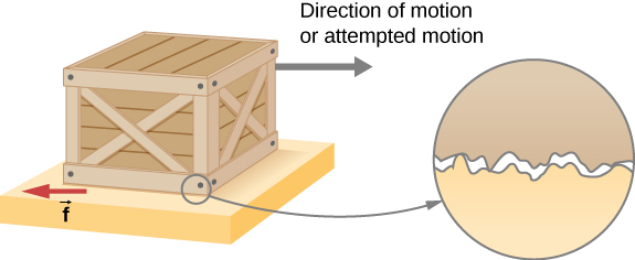
Figure 4.10 is a crude pictorial representation of how friction occurs at the interface between two objects. Close-up inspection of these surfaces shows them to be rough. Thus, when you push to get an object moving (in this case, a crate), you must raise the object until it can skip along with just the tips of the surface hitting, breaking off the points, or both. A considerable force can be resisted by friction with no apparent motion. The harder the surfaces are pushed together (such as if another box is placed on the crate), the more force is needed to move them. Part of the friction is due to adhesive forces between the surface molecules of the two objects, which explains the dependence of friction on the nature of the substances. For example, rubber-soled shoes slip less than those with leather soles. Adhesion varies with substances in contact and is a complicated aspect of forces between surfaces. Once an object is moving, there are fewer points of contact (fewer molecules adhering), so less force is required to keep the object moving. At small but nonzero speeds, friction is nearly independent of speed.
The size or magnitude of the frictional force has two forms: one for static situations (static friction), the other for situations involving motion (kinetic friction). What follows is an approximate (experimentally determined) model only. These equations for static and kinetic friction are not vector equations.
Static Friction
The magnitude of static friction [latex]{f}_{\text{s}}[/latex] is
[latex]{f}_{\text{s}}\le {\mu }_{\text{s}}N,[/latex]
where [latex]{\mu }_{\text{s}}[/latex] is the coefficient of static friction and N is the magnitude of the normal force.
The symbol [latex]\le[/latex] means less than or equal to, implying that static friction can have a maximum value of [latex]{\mu }_{\text{s}}N.[/latex] Static friction is a responsive force that increases to be equal and opposite to whatever force is exerted, up to its maximum limit. Once the applied force exceeds [latex]{f}_{\text{s}}\text{(max),}[/latex] the object moves. Thus,
[latex]{f}_{\text{s}}(\text{max})={\mu }_{\text{s}}N.[/latex]
Fs(max) is also referred to the maximum limiting friction.
Kinetic Friction
The magnitude of kinetic friction [latex]{f}_{\text{k}}[/latex] is given by
where [latex]{\mu }_{\text{k}}[/latex] is the coefficient of kinetic friction.
A system in which [latex]{f}_{\text{k}}={\mu }_{\text{k}}N[/latex] is described as a system in which friction behaves simply. The transition from static friction to kinetic friction is illustrated in Figure 4.11.
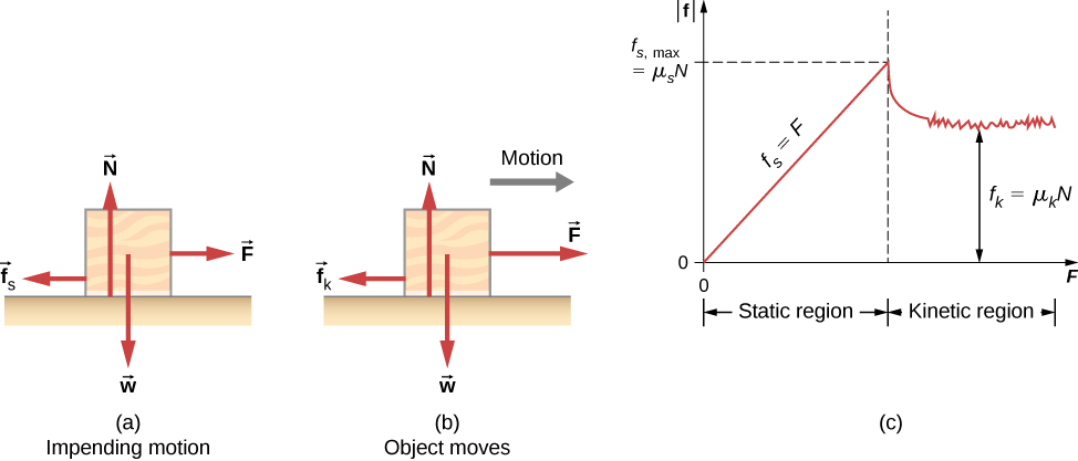
Table 6.1 below provides some examples of common coefficients of friction. As you can see, the coefficients of kinetic friction are less than their static counterparts. The approximate values of [latex]\mu[/latex] are stated to only one or two digits to indicate the approximate description of friction given by the preceding two equations.
| System | Static Friction [latex]{\mu }_{\text{s}}[/latex] | Kinetic Friction [latex]{\mu }_{\text{k}}[/latex] |
|---|---|---|
| Rubber on dry concrete | 1.0 | 0.7 |
| Rubber on wet concrete | 0.5-0.7 | 0.3-0.5 |
| Wood on wood | 0.5 | 0.3 |
| Waxed wood on wet snow | 0.14 | 0.1 |
| Metal on wood | 0.5 | 0.3 |
| Steel on steel (dry) | 0.6 | 0.3 |
| Steel on steel (oiled) | 0.05 | 0.03 |
| Teflon on steel | 0.04 | 0.04 |
| Bone lubricated by synovial fluid | 0.016 | 0.015 |
| Shoes on wood | 0.9 | 0.7 |
| Shoes on ice | 0.1 | 0.05 |
| Ice on ice | 0.1 | 0.03 |
| Steel on ice | 0.4 | 0.02 |
The equations for friction above include the dependence of friction on materials and the normal force. That is, the direction of friction is always opposite that of motion, parallel to the surface between objects, and perpendicular to the normal force. For example, if the crate you try to push (with a force parallel to the floor) has a mass of 100 kg, then the normal force is equal to its weight,
perpendicular to the floor. If the coefficient of static friction is 0.45, you would have to exert a force parallel to the floor greater than
[latex]{f}_{\text{s}}(\text{max})={\mu }_{\text{s}}N=(0.45)(980\,\text{N})=440\,\text{N}[/latex]
to move the crate. Once there is motion, friction is less and the coefficient of kinetic friction might be 0.30, so that a force of only
[latex]{f}_{\text{k}}={\mu }_{\text{k}}N=(0.30)(980\,\text{N})=290\,\text{N}[/latex]
keeps it moving at a constant speed. If the floor is lubricated, both coefficients are considerably less than they would be without lubrication. Coefficient of friction is a unitless quantity with a magnitude usually between 0 and 1.0. The actual value depends on the two surfaces that are in contact.
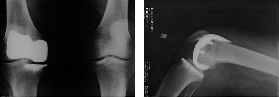
Many people have experienced the slipperiness of walking on ice. However, many parts of the body, especially the joints, have much smaller coefficients of friction—often three or four times less than ice. The ends of the bones in synovial joints, such as the knee or hip, are covered by cartilage, which provides a smooth, almost-glassy surface. The joints also produce a fluid (synovial fluid) that reduces friction and wear. A damaged or arthritic joint can be replaced by an artificial joint (Figure 4.12). These replacements can be made of metals (stainless steel or titanium) or plastic (polyethylene), also with very small coefficients of friction.
Similarly, natural lubricants in the body include saliva produced in our mouths to aid in the swallowing process, and the slippery mucus found between organs in the body, allowing them to move freely past each other during heartbeats, during breathing, and when a person moves. Hospitals and doctor’s clinics commonly use artificial lubricants, such as gels, to reduce friction. So there are abundant applications of friction in human movement.
Limitations to Friction Equations
The equations given for static and kinetic friction are empirical laws that describe the behavior of the forces of friction. While these formulas are very useful for practical purposes, they do not have the status of mathematical statements that represent general principles (e.g., Newton’s second law). In fact, there are cases for which these equations are not even good approximations. For instance, neither formula is accurate for lubricated surfaces or for two surfaces siding across each other at high speeds. Unless specified, we will not be concerned with these exceptions.
Example: Static and Kinetic Friction
A 20.0-kg crate is at rest on a floor as shown in Figure 4.13. The coefficient of static friction between the crate and floor is 0.700 and the coefficient of kinetic friction is 0.600. A horizontal force [latex]\overset{\to }{P}[/latex] is applied to the crate.
Find the force of friction if
(a) [latex]\overset{\to }{P}=20.0\,\text{N,}[/latex]
(b) [latex]\overset{\to }{P}=30.0\,\text{N,}[/latex]
(c) [latex]\overset{\to }{P}=120.0\,\text{N,}[/latex] and
(d) [latex]\overset{\to }{P}=180.0\,\text{N}\text{.}[/latex]
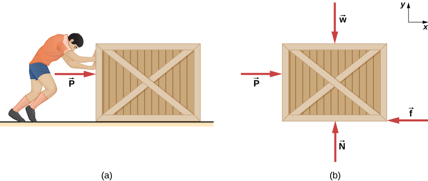
Strategy
The free-body diagram of the crate is shown in Figure 4.13(b). We apply Newton’s second law in the horizontal and vertical directions, including the friction force in opposition to the direction of motion of the box.
Solution
Newton’s second law gives
[latex]\begin{array}{cccc}\sum {F}_{x}=m{a}_{x}\hfill & & & \sum {F}_{y}=m{a}_{y}\hfill \\ P-f=m{a}_{x}\hfill & & & N-w=0.\hfill \end{array}[/latex]
Here we are using the symbol f to represent the frictional force since we have not yet determined whether the crate is subject to station friction or kinetic friction. We do this whenever we are unsure what type of friction is acting. Now the weight of the crate is
[latex]w=(20.0\,\text{kg})(9.80\,{\text{m/s}}^{2})=196\,\text{N,}[/latex]
which is also equal to N. The maximum force of static friction is therefore:
[latex](0.700)(196\,\text{N})=137\,\text{N}\text{.}[/latex]
As long as [latex]\overset{\to }{P}[/latex] is less than 137 N, the force of static friction keeps the crate stationary and [latex]{f}_{\text{s}}=\overset{\to }{P}.[/latex]
Thus, (a) [latex]{f}_{s}=20.0\,\text{N,}[/latex]
(b) [latex]{f}_{s}=30.0\,\text{N,}[/latex] and
(c) [latex]{f}_{s}=120.0\,\text{N}\text{.}[/latex]
(d) This is a more advanced example, but we can work through it by carefully applying the principles we've learned so far. If [latex]\overset{\to }{P}=180.0\,\text{N,}[/latex] the applied force is greater than the maximum force of static friction (137 N), so the crate can no longer remain at rest. Once the crate is in motion, kinetic friction acts. Then
[latex]{f}_{\text{k}}={\mu }_{\text{k}}N=(0.600)(196\,\text{N})=118\,\text{N,}[/latex]
and the acceleration is
[latex]{a}_{x}=\frac{\overset{\to }{P}-{f}_{\text{k}}}{m}=\frac{180.0\,\text{N}-118\,\text{N}}{20.0\,\text{kg}}=3.10\,{\text{m/s}}^{2}\text{.}[/latex]
Discussion
This example illustrates how we consider friction in a dynamics problem. Notice that static friction has a value that matches the applied force, until we reach the maximum value of static friction. Also, no motion can occur until the applied force equals the force of static friction, but the force of kinetic friction will then become smaller.
Check your Understanding
A block of mass 1.0 kg rests on a horizontal surface. The frictional coefficients for the block and surface are [latex]{\mu }_{s}=0.50[/latex] and [latex]{\mu }_{k}=0.40.[/latex]
(a) What is the minimum horizontal force required to move the block?
(b) What is the block’s acceleration when this force is applied?
Solution:
a. 4.9 N;
b. 0.98 m/s2
Friction and the Inclined Plane
One situation where friction plays an obvious role is that of an object on a slope. It might be a crate being pushed up a ramp to a loading dock or a skateboarder coasting down a mountain, but the basic biomechanics is the same. We usually generalize the sloping surface and call it an inclined plane but then pretend that the surface is flat. Let’s look at an example of analyzing motion on an inclined plane with friction.
Example: Downhill Skier
A skier with a mass of 62 kg is sliding down a snowy slope at a constant velocity. Find the coefficient of kinetic friction for the skier if friction is known to be 45.0 N.
Strategy
The magnitude of kinetic friction is given as 45.0 N. Kinetic friction is related to the normal force [latex]N[/latex] by
[latex]{f}_{\text{k}}={\mu }_{\text{k}}N[/latex];
thus, we can find the coefficient of kinetic friction if we can find the normal force on the skier. The normal force is always perpendicular to the surface, and since there is no motion perpendicular to the surface, the normal force should equal the component of the skier’s weight perpendicular to the slope. (See Figure 4.14, which repeats a figure from the chapter on Newton’s laws of motion.)
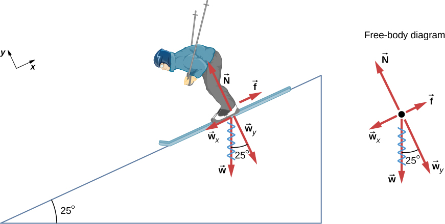
We have
[latex]N={w}_{y}=w\,\text{cos}\,25\text{°}=mg\,\text{cos}\,25\text{°}.[/latex]
Substituting this into our expression for kinetic friction, we obtain
[latex]{f}_{\text{k}}={\mu }_{\text{k}}mg\,\text{cos}\,25\text{°},[/latex]
which can now be solved for the coefficient of kinetic friction [latex]{\mu }_{\text{k}}.[/latex]
Solution
Solving for [latex]{\mu }_{\text{k}}[/latex] gives
[latex]{\mu }_{\text{k}}=\frac{{f}_{\text{k}}}{N}=\frac{{f}_{\text{k}}}{w\,\text{cos}\,25\text{°}}=\frac{{f}_{\text{k}}}{mg\,\text{cos}\,25\text{°}}.[/latex]
Substituting known values on the right-hand side of the equation,
[latex]{\mu }_{\text{k}}=\frac{45.0\,\text{N}}{(62\,\text{kg})(9.80\,{\text{m/s}}^{2})(0.906)}=0.082.[/latex]
Discussion
This result is a little smaller than the coefficient listed in Table 6.1 for waxed wood on snow, but it is still reasonable since values of the coefficients of friction can vary greatly. In situations like this, where an object of mass m slides down a slope that makes an angle [latex]\theta[/latex] with the horizontal, friction is given by [latex]{f}_{\text{k}}={\mu }_{\text{k}}mg\,\text{cos}\,\theta .[/latex] All objects slide down a slope with constant acceleration under these circumstances.
Calculating Coefficients of Friction
We have discussed that when an object rests on a horizontal surface, the normal force supporting it is equal in magnitude to its weight. Furthermore, simple friction is always proportional to the normal force. When an object is not on a horizontal surface, as with the inclined plane, we must find the force acting on the object that is directed perpendicular to the surface; it is a component of the weight.
We now derive a useful relationship for calculating coefficient of friction on an inclined plane. Notice that the result applies only for situations in which the object slides at constant speed down the ramp.
An object slides down an inclined plane at a constant velocity if the net force on the object is zero. We can use this fact to measure the coefficient of kinetic friction between two objects. As shown in the example above, the kinetic friction on a slope is [latex]{f}_{k}={\mu }_{k}mg\,\text{cos}\,\theta[/latex]. The component of the weight down the slope is equal to [latex]mg\,\text{sin}\,\theta[/latex] (see the free-body diagram in Figure 4.14). These forces act in opposite directions, so when they have equal magnitude, the acceleration is zero. Writing these out,
[latex]{\mu }_{\text{k}}mg\,\text{cos}\,\theta =mg\,\text{sin}\,\theta .[/latex]
Solving for [latex]{\mu }_{\text{k}},[/latex] we find that
[latex]{\mu }_{\text{k}}=\frac{mg\,\text{sin}\,\theta }{mg\,\text{cos}\,\theta }=\text{tan}\,\theta .[/latex]
Put a coin on a book and tilt it until the coin slides at a constant velocity down the book. You might need to tap the book lightly to get the coin to move. Measure the angle of tilt relative to the horizontal and find [latex]{\mu }_{\text{k}}.[/latex] Note that the coin does not start to slide at all until an angle greater than [latex]\theta[/latex] is attained, since the coefficient of static friction is larger than the coefficient of kinetic friction. Think about how this may affect the value for [latex]{\mu }_{\text{k}}[/latex] and its uncertainty.
Advanced Topic: Atomic-Scale Explanations of Friction
The simpler aspects of friction dealt with so far are its macroscopic (large-scale) characteristics. Great strides have been made in the atomic-scale explanation of friction during the past several decades. Researchers are finding that the atomic nature of friction seems to have several fundamental characteristics. These characteristics not only explain some of the simpler aspects of friction—they also hold the potential for the development of nearly friction-free environments that could save hundreds of billions of dollars in energy which is currently being converted (unnecessarily) into heat.
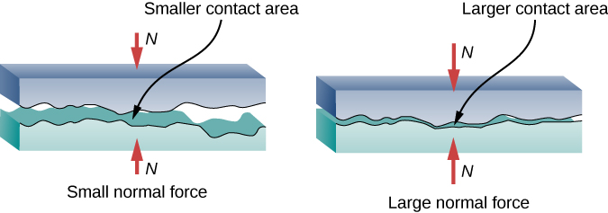
Figure 4.15 illustrates one macroscopic characteristic of friction that is explained by microscopic (small-scale) research. We have noted that friction is proportional to the normal force, but not to the amount of area in contact, a somewhat counterintuitive notion. When two rough surfaces are in contact, the actual contact area is a tiny fraction of the total area because only high spots touch. When a greater normal force is exerted, the actual contact area increases, and we find that the friction is proportional to this area.
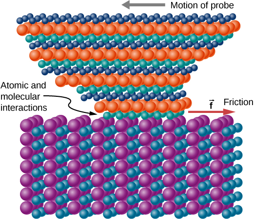
However, the atomic-scale view promises to explain far more than the simpler features of friction. The mechanism for how heat is generated is now being determined. In other words, why do surfaces get warmer when rubbed? Essentially, atoms are linked with one another to form lattices. When surfaces rub, the surface atoms adhere and cause atomic lattices to vibrate—essentially creating sound waves that penetrate the material. The sound waves diminish with distance, and their energy is converted into heat. Chemical reactions that are related to frictional wear can also occur between atoms and molecules on the surfaces. Figure 4.16 shows how the tip of a probe drawn across another material is deformed by atomic-scale friction. The force needed to drag the tip can be measured and is found to be related to shear stress, which is discussed in a later chapter. The variation in shear stress is remarkable (more than a factor of [latex]{10}^{12}[/latex]) and difficult to predict theoretically, but shear stress is yielding a fundamental understanding of a large-scale phenomenon known since ancient times—friction.
Example: Snowboarding
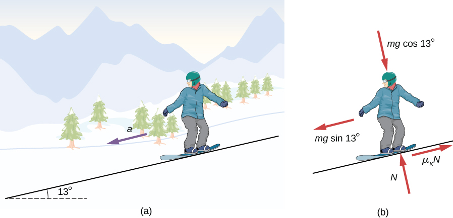
Earlier, we analyzed the situation of a downhill skier moving at constant velocity to determine the coefficient of kinetic friction. Now let’s do a similar analysis to determine acceleration. The snowboarder of FIgure 4.19 glides down a slope that is inclined at [latex]\theta ={13}^{0}[/latex] to the horizontal. The coefficient of kinetic friction between the board and the snow is [latex]{\mu }_{\text{k}}=0.20.[/latex]
What is the acceleration of the snowboarder?
Strategy
The forces acting on the snowboarder are her weight and the contact force of the slope, which has a component normal to the incline and a component along the incline (force of kinetic friction). Because she moves along the slope, the most convenient reference frame for analyzing her motion is one with the x-axis along and the y-axis perpendicular to the incline. In this frame, both the normal and the frictional forces lie along coordinate axes, the components of the weight are [latex]mg\,\text{sin}\,\theta[/latex] along the slope and [latex]\,mg\,\text{cos}\,\theta[/latex] at right angles into the slope, and the only acceleration is along the x-axis [latex]({a}_{y}=0).[/latex]
Solution
We can now apply Newton’s second law to the snowboarder:
[latex]\begin{array}{cccccc}\hfill \sum {F}_{x}& =\hfill & m{a}_{x}\hfill & & & \sum {F}_{y}=m{a}_{y}\hfill \\ \hfill mg\,\text{sin}\,\theta -{\mu }_{k}N& =\hfill & m{a}_{x}\hfill & & & \hfill N-mg\,\text{cos}\,\theta =m(0)\text{.}\end{array}[/latex]
From the second equation, [latex]N=mg\,\text{cos}\,\theta . [latex] Upon substituting this into the first equation, we find
[latex]\begin{array}{cc}\hfill {a}_{x}& =g(\text{sin}\,\theta -{\mu }_{\text{k}}\,\text{cos}\,\theta )\hfill \\ & =g(\text{sin}\,13\text{°}-0.20\,\text{cos}\,13\text{°})=0.29\,{\text{m/s}}^{2}\text{.}\hfill \end{array}[/latex]
Discussion
Notice from this equation that if [latex]\theta[/latex] is small enough or [latex]{\mu }_{\text{k}}[/latex] is large enough, [latex]{a}_{x}[/latex] is negative, that is, the snowboarder slows down.
Check your Understanding
The snowboarder is now moving down a hill with incline [latex]10.0\text{°}[/latex]. What is the skier’s acceleration?
Solution:
[latex]\text{−0.23}\,{\text{m/s}}^{2}[/latex]; the negative sign indicates that the snowboarder is slowing down.
Example: A Crate on an Accelerating Truck
A 50.0-kg crate rests on the bed of a truck as shown in Figure 4.18. The coefficients of friction between the surfaces are [latex]{\mu }_{\text{k}}=0.300[/latex] and [latex]{\mu }_{\text{s}}=0.400.[/latex] Find the frictional force on the crate when the truck is accelerating forward relative to the ground at
(a) 2.00 m/s2, and
(b) 5.00 m/s2.
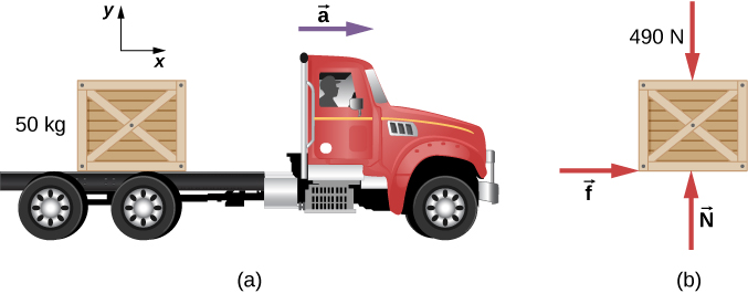
Strategy
The forces on the crate are its weight and the normal and frictional forces due to contact with the truck bed. We start by assuming that the crate is not slipping. In this case, the static frictional force [latex]{f}_{\text{s}}[/latex] acts on the crate. Furthermore, the accelerations of the crate and the truck are equal.
Solution
(a) Application of Newton’s second law to the crate, using the reference frame attached to the ground, yields
[latex]\begin{array}{cccccccc}\hfill \sum {F}_{x}& =\hfill & m{a}_{x}\hfill & & & \hfill \sum {F}_{y}& =\hfill & m{a}_{y}\hfill \\ \hfill {f}_{\text{s}}& =\hfill & (50.0\,\text{kg})(2.00\,{\text{m/s}}^{2})\hfill & & & \hfill N-4.90\,×\,{10}^{2}\,\text{N}& =\hfill & (50.0\,\text{kg})(0)\hfill \\ & =\hfill & 1.00\,×\,{10}^{2}\,\text{N}\hfill & & & \hfill N& =\hfill & 4.90\,×\,{10}^{2}\,\text{N}\text{.}\hfill \end{array}[/latex]
We can now check the validity of our no-slip assumption. The maximum value of the force of static friction is
whereas the actual force of static friction that acts when the truck accelerates forward at [latex]2.00\,{\text{m/s}}^{2}[/latex] is only [latex]1.00\,×\,{10}^{2}\,\text{N}\text{.}[/latex] Thus, the assumption of no slipping is valid.
(b) If the crate is to move with the truck when it accelerates at [latex]5.0\,{\text{m/s}}^{2},[/latex] the force of static friction must be
[latex]{f}_{\text{s}}=m{a}_{x}=(50.0\,\text{kg})(5.00\,{\text{m/s}}^{2})=250\,\text{N}\text{.}[/latex]
Since this exceeds the maximum of 196 N, the crate must slip. The frictional force is therefore kinetic and is
The horizontal acceleration of the crate relative to the ground is now found from
Discussion
Relative to the ground, the truck is accelerating forward at [latex]5.0\,{\text{m/s}}^{2}[/latex] and the crate is accelerating forward at [latex]2.94\,{\text{m/s}}^{2}[/latex]. Hence the crate is sliding backward relative to the bed of the truck with an acceleration [latex]2.94\,{\text{m/s}}^{2}-5.00\,{\text{m/s}}^{2}=-2.06\,{\text{m/s}}^{2}\text{.}[/latex]
