3.3 Adding and Subtracting Vectors: Algebra

Rob Pryce

Chapter 3 Describing Movement in Two Dimensions, 2-D Linear Kinematics

3.3 Adding and Subtracting Vectors: Algebra

Authors: Paul Peter Urone, Roger Hinrichs
Adapted by: Rob Pryce, Alix Blacklin

Learning Objectives

By the end of this section, you will be able to:

Understand the rules of vector addition and subtraction using analytical methods.
Apply analytical methods to determine vertical and horizontal component vectors.
Apply analytical methods to determine the magnitude and direction of a resultant vector.

Analytical methods of vector addition and subtraction employ geometry and simple trigonometry rather than the ruler and protractor of graphical methods. Part of the graphical technique is retained, because vectors are still represented by arrows for easy visualization. However, analytical methods are more concise, accurate, and precise than graphical methods, which are limited by the accuracy with which a drawing can be made. Analytical methods are limited only by the accuracy and precision with which physical quantities are known.

Resolving a Vector into Its Components

Analytical techniques and right triangles go hand-in-hand in biomechanics because (among other things) motions along perpendicular directions are independent. We very often need to separate a vector into its perpendicular components. For example, given a vector like [latex]\vec{A}[/latex] in Figure 3.24, we may wish to find which two perpendicular vectors, [latex]\vec{A_x}[/latex]) and [latex]\vec{A_y}[/latex], add to produce it.

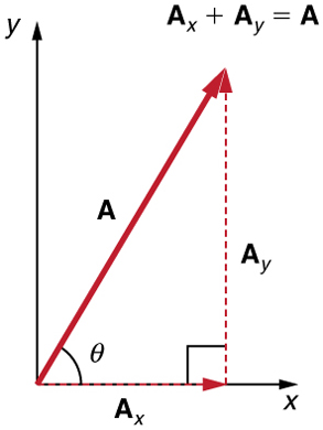
In the given figure a dotted vector A sub x is drawn from the origin along the x axis. From the head of the vector A sub x another vector A sub y is drawn in the upward direction. Their resultant vector A is drawn from the tail of the vector A sub x to the head of the vector A sub y at an angle theta from the x axis. On the graph a vector A, inclined at an angle theta with x axis is shown. Therefore vector A is the sum of the vectors A sub x and A sub y. — Figure 3.24 The vector [latex]\vec{A}[/latex], with its tail at the origin of an x, y-coordinate system, is shown together with its x- and y-components, [latex]\vec{A_x}[/latex]) and [latex]\vec{A_y}[/latex]. These vectors form a right triangle. The analytical relationships among these vectors are summarized below.

[latex]\vec{A_x}[/latex] and [latex]\vec{A_y}[/latex] are defined to be the components of [latex]\vec{A}[/latex] along the x– and y-axes. The three vectors [latex]\vec{A}[/latex], [latex]\vec{A_x}[/latex], and [latex]\vec{A_y}[/latex] form a right triangle:

[latex]\vec{A_x} + \vec{A_y} = \vec{A}[/latex]

Note that this relationship between components of the vector and the resultant holds only for vector quantities (which include both magnitude and direction). The relationship does not apply for the magnitudes alone. For example, if [latex]\vec{A_x}=\text{3 m east}[/latex], [latex]\vec{A_y}=\text{4 m north}[/latex], and [latex]\vec{A}=\text{5 m north-east}[/latex], then it is true that the vectors [latex]\vec{A_x} + \vec{A_y} = \vec{A}[/latex]. However, it is not true that the sum of the magnitudes of the vectors is also equal. That is,

[latex]\text{3m} + \text{4m} \ne \text{5m}[/latex]

Thus,

[latex]\textit{A}_x + \textit{A}_y \ne \textit{A}[/latex]

If the vector [latex]\vec{A}[/latex] is known, then its magnitude [latex]\textit{A}[/latex] (its length) and its angle [latex]\theta[/latex] (its direction) are known. To find [latex]\vec{A_x}[/latex] and [latex]\vec{A_y}[/latex], its x- and y-components, we use the following relationships for a right triangle.

[latex]\vec{A_x}=A\phantom{\rule{0.25em}{0ex}}\text{cos}\phantom{\rule{0.25em}{0ex}}\theta[/latex]

and

[latex]\vec{A_y}=A\phantom{\rule{0.25em}{0ex}}\text{sin}\phantom{\rule{0.25em}{0ex}}\theta \text{.}[/latex]

]A dotted vector A sub x whose magnitude is equal to A cosine theta is drawn from the origin along the x axis. From the head of the vector A sub x another vector A sub y whose magnitude is equal to A sine theta is drawn in the upward direction. Their resultant vector A is drawn from the tail of the vector A sub x to the head of the vector A-y at an angle theta from the x axis. Therefore vector A is the sum of the vectors A sub x and A sub y. — Figure 3.25 The magnitudes of the vector components [latex]\vec{A_x}[/latex] and [latex]\vec{A_y}[/latex] can be related to the resultant vector [latex]\vec{A}[/latex] and the angle [latex]\theta[/latex] with trigonometry. Here we see that [latex]\vec{A_x}=A\phantom{\rule{0.25em}{0ex}}\text{cos}\phantom{\rule{0.25em}{0ex}}\theta [/latex] and [latex]\vec{A_y}=A\phantom{\rule{0.25em}{0ex}}\text{sin}\phantom{\rule{0.25em}{0ex}}\theta [/latex].

Suppose, for example, that [latex]\vec{A}[/latex] is the vector representing the total displacement of the person walking in a city considered in the previous two sections.

In the given figure a vector A of magnitude ten point three blocks is inclined at an angle twenty nine point one degrees to the positive x axis. The horizontal component A sub x of vector A is equal to A cosine theta which is equal to ten point three blocks multiplied to cosine twenty nine point one degrees which is equal to nine blocks east. Also the vertical component A sub y of vector A is equal to A sin theta is equal to ten point three blocks multiplied to sine twenty nine point one degrees, which is equal to five point zero blocks north. — Figure 3.26 We can use the relationships [latex]\vec{A_x}=A\phantom{\rule{0.25em}{0ex}}\text{cos}\phantom{\rule{0.25em}{0ex}}\theta [/latex] and [latex]\vec{A_y}=A\phantom{\rule{0.25em}{0ex}}\text{sin}\phantom{\rule{0.25em}{0ex}}\theta [/latex] to determine the magnitude of the horizontal and vertical component vectors in this example.

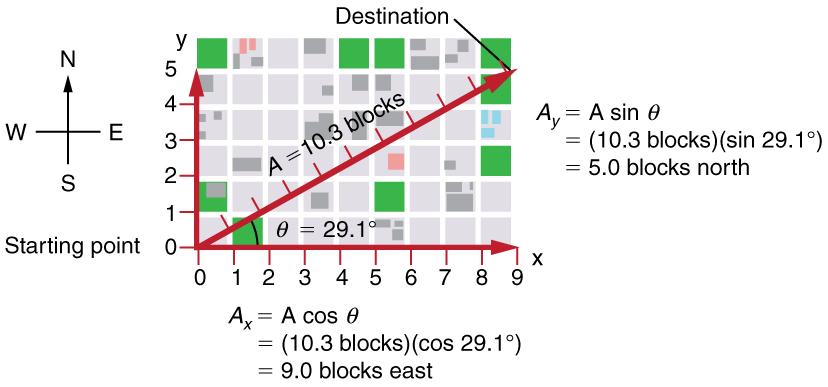
Then [latex]\textit{A}=10.3[/latex] blocks and [latex]\theta =29.1º[/latex] , so that

[latex]\vec{A_x}=A\phantom{\rule{0.25em}{0ex}}\text{cos}\phantom{\rule{0.25em}{0ex}}\theta =\left(\text{10.3 blocks}\right)\left(\text{cos}\phantom{\rule{0.25em}{0ex}}29.1º\right)=\text{9.0 blocks}[/latex]

[latex]\vec{A_y}=A\phantom{\rule{0.25em}{0ex}}\text{sin}\phantom{\rule{0.25em}{0ex}}\theta =\left(\text{10.3 blocks}\right)\left(\text{sin}\phantom{\rule{0.25em}{0ex}}29.1º\right)=\text{5.0 blocks}\text{.}[/latex]

Calculating a Resultant Vector

If the perpendicular components [latex]\vec{A_x}[/latex] and [latex]\vec{A_y}[/latex] of a vector [latex]\vec{A}[/latex] are known, then [latex]\vec{A}[/latex] can also be found by calculation. To find the magnitude [latex]\textit{A}[/latex] and direction [latex]\theta[/latex] of a vector from its perpendicular components [latex]\vec{A_x}[/latex] and [latex]\vec{A_y}[/latex], we use the following relationships:

[latex]\textit{A}=\sqrt{\textit{A}_x^{2}+\textit{A}_y^{2}}[/latex]

[latex]\theta ={\text{tan}}^{-1}\frac{\textit{A}_y}{\textit{A}_x}[/latex]

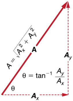
Vector A is shown with its horizontal and vertical components A sub x and A sub y respectively. The magnitude of vector A is equal to the square root of A sub x squared plus A sub y squared. The angle theta of the vector A with the x axis is equal to inverse tangent of A sub y over A sub x — Figure 3.27 The magnitude and direction of the resultant vector can be determined once the horizontal and vertical components [latex]\vec{A_x}[/latex] and [latex]\vec{A_y}[/latex] have been determined.

Note that the equation [latex]\textit{A}=\sqrt{\textit{A}_x^{2}+\textit{A}_y^{2}}[/latex] is just the Pythagorean theorem relating the legs of a right triangle to the length of the hypotenuse. For example, if [latex]\vec{A_x}[/latex] and [latex]\vec{A_y}[/latex] are 9 and 5 blocks, respectively, then [latex]\textit{A}=\sqrt{{9}^{2}{\text{+5}}^{2}}\text{=10}\text{.}3[/latex] blocks, again consistent with the example of the person walking in a city. Finally, the direction is [latex]\theta ={\text{tan}}^{–1}\left(\text{5/9}\right)=29.1º[/latex] , as before.

Determining Vectors and Vector Components with Analytical Methods

Equations [latex]\textit{A}_x=\textit{A}\phantom{\rule{0.25em}{0ex}}\text{cos}\phantom{\rule{0.25em}{0ex}}\theta[/latex] and [latex]\textit{A_y}=A\phantom{\rule{0.25em}{0ex}}\text{sin}\phantom{\rule{0.25em}{0ex}}\theta[/latex] are used to find the perpendicular components of a vector—that is, to go from it’s magnitude, [latex]\textit{A}[/latex], and direction, [latex]\theta[/latex], to its components, [latex]\textit{A}_x[/latex] and [latex]\textit{A}_y[/latex].

Equations [latex]\textit{A}=\sqrt{\textit{A_x}^{2}+\textit{A_y}^{2}}[/latex] and [latex]\theta ={\text{tan}}^{\text{–1}}\left(\textit{A}_y/\textit{A}_x\right)[/latex] are used to find a vector from its perpendicular components—that is, to go from [latex]\textit{A}_x[/latex] and [latex]\textit{A}_y[/latex] to [latex]\textit{A}[/latex] and [latex]\theta[/latex].

Both processes are crucial to analytical methods of vector addition and subtraction.

Adding Multiple Vectors Using Analytical Methods

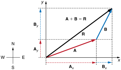
To see how to add vectors using perpendicular components, consider Figure 3.28, in which the vectors [latex]\vec{A}[/latex] and [latex]\vec{B}[/latex] are added to produce the resultant [latex]\vec{R}[/latex].

Two vectors A and B are shown. The tail of vector B is at the head of vector A and the tail of the vector A is at origin. Both the vectors are in the first quadrant. The resultant R of these two vectors extending from the tail of vector A to the head of vector B is also shown. — Figure 3.28 Vectors [latex]\vec{A}[/latex] and [latex]\vec{B}[/latex] are two legs of a walk, and [latex]\vec{R}[/latex] is the resultant or total displacement. You can use analytical methods to determine the magnitude and direction of [latex]\vec{R}[/latex].

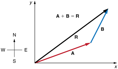
If [latex]\vec{A}[/latex] and [latex]\vec{B}[/latex] represent two legs of a walk (two displacements), then [latex]\vec{R}[/latex] is the total displacement. The person taking the walk ends up at the tip of [latex]\vec{R}[/latex]. There are many ways to arrive at the same point. In particular, the person could have walked first in the x-direction and then in the y-direction. Those paths are the x– and y-components of the resultant, [latex]\vec{R}_x[/latex] and [latex]\vec{R}_y[/latex].

If we know [latex]\vec{R}_x[/latex] and [latex]\vec{R}_y[/latex], we can find [latex]\textit{R}[/latex] and [latex]\theta[/latex] using the equations:

[latex]\textit{A}=\sqrt{\textit{A}_x^{2}+\textit{A}_y^{2}}[/latex] and

[latex]\theta ={\text{tan}}^{–1}\left(\textit{A}_y/\textit{A}_x\right)[/latex].

When you use the analytical method of vector addition, you can determine the components or the magnitude and direction of a vector.

Step 1. Identify the x- and y-axes that will be used in the problem. Then, find the components of each vector to be added along the chosen perpendicular axes. Use the equations:

[latex]\textit{A}_x=A\phantom{\rule{0.25em}{0ex}}\text{cos}\phantom{\rule{0.25em}{0ex}}\theta[/latex] and

[latex]\textit{A}_y=A\phantom{\rule{0.25em}{0ex}}\text{sin}\phantom{\rule{0.25em}{0ex}}\theta[/latex] to find the components.

In Figure 3.29, these components are [latex]\textit{A}_x[/latex], [latex]\textit{A}_y[/latex], [latex]\textit{B}_x[/latex], and [latex]\textit{B}_y[/latex]. The angles that vectors [latex]\vec{A}[/latex] and [latex]\vec{B}[/latex] make with the x-axis are [latex]\theta_A[/latex] and [latex]\theta_B[/latex], respectively.

Two vectors A and B are shown. The tail of the vector B is at the head of vector A and the tail of the vector A is at origin. Both the vectors are in the first quadrant. The resultant R of these two vectors extending from the tail of vector A to the head of vector B is also shown. The horizontal and vertical components of the vectors A and B are shown with the help of dotted lines. The vectors labeled as A sub x and A sub y are the components of vector A, and B sub x and B sub y as the components of vector B.. — Figure 3.29 To add vectors [latex]\vec{A}[/latex] and [latex]\vec{B}[/latex], first determine the horizontal and vertical components of each vector. These are the vectors indicated by the dotted lines: [latex]\vec{A_x}, \vec{A_y}, \vec{B_x}, \text{and} \vec{B_y}[/latex] shown in the image above.

Step 2. Find the components of the resultant along each axis by adding the components of the individual vectors along that axis. That is, as shown in Figure 3.30,

[latex]\textit{R}_x=\textit{A}_x+\textit{B}_x[/latex]

and

[latex]\textit{R}_y=\textit{A}_y+\textit{B}_y[/latex]

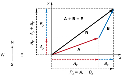
Components along the same axis, say the x-axis, are vectors along the same line and, thus, can be added to one another like ordinary numbers. The same is true for components along the y-axis. (For example, a 9-block eastward walk could be taken in two legs, the first 3 blocks east and the second 6 blocks east, for a total of 9, because they are along the same direction.) So resolving vectors into components along common axes makes it easier to add them. Now that the components of [latex]\vec{R}[/latex] are known, its magnitude and direction can be found.

Step 3. To get the magnitude [latex]\textit{R}[/latex] of the resultant, use the Pythagorean theorem:

[latex]\textit{R}=\sqrt{\textit{R}_x^{2}+\textit{R}_y^{2}}\text{.}[/latex]

Step 4. To get the direction of the resultant:

[latex]\theta ={\text{tan}}^{-1}\left(\textit{R}_y/\textit{R}_x\right)\text{.}[/latex]

The following example illustrates this technique for adding vectors using perpendicular components.

Example: Adding Multiple Vectors Using Analytical Methods

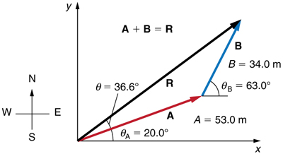
Add the vector [latex]\vec{A}[/latex] to the vector [latex]\vec{B}[/latex] shown in Figure 3.31, using perpendicular components along the x– and y-axes. The x– and y-axes are along the east–west and north–south directions, respectively. Vector [latex]\vec{A}[/latex] represents the first leg of a walk in which a person walks 53.0 m in a direction 20.0º north of east. Vector [latex]\vec{B}[/latex] represents the second leg, a displacement of 34.0 m in a direction 63.0º north of east.

Two vectors A and B are shown. The tail of the vector A is at origin. Both the vectors are in the first quadrant. Vector A is of magnitude fifty three units and is inclined at an angle of twenty degrees to the horizontal. From the head of the vector A another vector B of magnitude 34 units is drawn and is inclined at angle sixty three degrees with the horizontal. The resultant of two vectors is drawn from the tail of the vector A to the head of the vector B. — Figure 3.31 Vector [latex]\vec{A}[/latex] has magnitude 53.0m and direction 20.0º north of the x-axis. Vector [latex]\vec{B}[/latex] has magnitude 34.0m and direction 63.0º north of the x-axis. You can use analytical methods to determine the magnitude and direction of [latex]\vec{R}[/latex].

Strategy

The components of [latex]\vec{A}[/latex] and [latex]\vec{B}[/latex] along the x– and y-axes represent walking due east and due north to get to the same ending point. Once found, they are combined to produce the resultant.

Solution

Following the method outlined above, we first find the components of [latex]\vec{A}[/latex] and [latex]\vec{B}[/latex] along the x– and y-axes. Note that
[latex]\textit{A} = \text{53.0 m}[/latex],
[latex]\theta_A=20.0º[/latex],
[latex]\textit{B}=\text{34.0 m}[/latex], and
[latex]\theta_B=\text{63.0º}[/latex].

We find the x-components by using [latex]\textit{A}_x=\textit{A}\phantom{\rule{0.25em}{0ex}}\text{cos}\phantom{\rule{0.25em}{0ex}}\theta[/latex], which gives:

[latex]\begin{array}{lll}{A}_{x}& =& A\phantom{\rule{0.25em}{0ex}}\text{cos}\phantom{\rule{0.25em}{0ex}}{\theta }_{A}=\left(\text{53.}0 m\text{}\right)\left(\text{cos 20.0º}\right)\\ & =& \left(\text{53.}0 m\right)\left(0\text{.940}\right)=\text{49.}8 m\end{array}[/latex]

and

[latex]\begin{array}{lll}{B}_{x}& =& B\phantom{\rule{0.25em}{0ex}}\text{cos}\phantom{\rule{0.25em}{0ex}}{\theta }_{B}=\left(\text{34}\text{.}0 m\text{}\right)\left(\text{cos 63.0º}\right)\\ & =& \text{}\left(\text{34}\text{.}0 m\text{}\right)\left(0\text{.}\text{454}\right)=\text{15}\text{.}4 m\text{.}\end{array}[/latex]

Similarly, the y-components are found using [latex]{A}_{y}=A\phantom{\rule{0.25em}{0ex}}\text{sin}\phantom{\rule{0.25em}{0ex}}{\theta }_{A}[/latex]

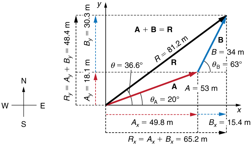
[latex]\begin{array}{lll}{A}_{y}& =& A\phantom{\rule{0.25em}{0ex}}\text{sin}\phantom{\rule{0.25em}{0ex}}{\theta }_{A}=\left(\text{53}\text{.}0 m\text{}\right)\left(\text{sin 20.0º}\right)\\ & =& \text{}\left(\text{53}\text{.}0 m\text{}\right)\left(0\text{.}\text{342}\right)=\text{18}\text{.}1 m\text{}\end{array}[/latex]

and

[latex]\begin{array}{lll}{B}_{y}& =& B\phantom{\rule{0.25em}{0ex}}\text{sin}\phantom{\rule{0.25em}{0ex}}{\theta }_{B}=\left(\text{34}\text{.}0 m\text{}\right)\left(\text{sin 63}\text{.}0º\right)\\ & =& \text{}\left(\text{34}\text{.}0 m\text{}\right)\left(0\text{.}\text{891}\right)=\text{30}\text{.}3 m\text{}\text{.}\end{array}[/latex]

The x– and y-components of the resultant are thus

[latex]{R}_{x}={A}_{x}+{B}_{x}=\text{49}\text{.}8 m\text{}+\text{15}\text{.}4 m\text{}=\text{65}\text{.}2 m\text{}[/latex]

and

[latex]{R}_{y}={A}_{y}+{B}_{y}=\text{18}\text{.}1 m+\text{30}\text{.}3 m=\text{48}\text{.}4 m\text{.}[/latex]

Now we can find the magnitude of the resultant by using the Pythagorean theorem:

[latex]R=\sqrt{{R}_{x}^{2}+{R}_{y}^{2}}=\sqrt{65.2^2+48.4^2}[/latex]

so that

[latex]R=81.2 m.\text{}[/latex]

Finally, we find the direction of the resultant:

[latex]\theta ={\text{tan}}^{-1}\left({R}_{y}/{R}_{x}\right)\text{=}{\text{tan}}^{-1}\left(\text{48}\text{.}4/\text{65}\text{.}2\right)\text{.}[/latex]

Thus,

[latex]\theta ={\text{tan}}^{-1}\left(0\text{.}\text{742}\right)=\text{36}\text{.}6º\text{.}[/latex]

The addition of two vectors A and B is shown. Vector A is of magnitude fifty three units and is inclined at an angle of twenty degrees to the horizontal. Vector B is of magnitude thirty four units and is inclined at angle sixty three degrees to the horizontal. The components of vector A are shown as dotted vectors A X is equal to forty nine point eight meter along x axis and A Y is equal to eighteen point one meter along Y axis. The components of vector B are also shown as dotted vectors B X is equal to fifteen point four meter and B Y is equal to thirty point three meter. The horizontal component of the resultant R X is equal to A X plus B X is equal to sixty five point two meter. The vertical component of the resultant R Y is equal to A Y plus B Y is equal to forty eight point four meter. The magnitude of the resultant of two vectors is eighty one point two meters. The direction of the resultant R is in thirty six point six degree from the vector A in anticlockwise direction. — Figure 3.32 Using analytical methods, we see that the magnitude of [latex]\vec{R}[/latex] is 81.2 m and its direction is 36.6º north of east.

Discussion

This example illustrates the addition of vectors using perpendicular components. Vector subtraction using perpendicular components is very similar—it is just the addition of a negative vector.

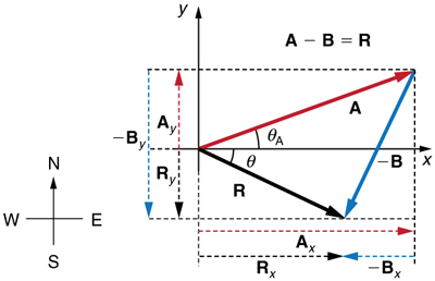
Subtraction of vectors is accomplished by the addition of a negative vector. That is, [latex]\vec{A}-\vec{B}\equiv \vec{A}+\left(\vec{–B}\right)[/latex]. Thus, the method for the subtraction of vectors using perpendicular components is identical to that for addition. The components of [latex]\vec{–B}[/latex] are the negatives of the components of [latex]\vec{B}[/latex].

The x– and y-components of the resultant [latex]\vec{A}-\vec{B} =\vec{R}[/latex]) are thus

[latex]\textit{R}_x=\textit{A}_x+\left(–\textit{B}_x\right)[/latex]

and

[latex]\textit{R}_y=\textit{A}_y+\left(–\textit{B}_y\right)[/latex]

and the rest of the method outlined above is identical to that for addition. (See Figure 3.33)

Analyzing vectors using perpendicular components is very useful in many areas of biomechanics, because perpendicular quantities are often independent of one another. The next module, Projectile Motion, is one of many in which using perpendicular components helps make the picture clear and simplifies the underlying biomechanics.

In this figure, the subtraction of two vectors A and B is shown. A red colored vector A is inclined at an angle theta A to the positive of x axis. From the head of vector A a blue vector negative B is drawn. Vector B is in west of south direction. The resultant of the vector A and vector negative B is shown as a black vector R from the tail of vector A to the head of vector negative B. The resultant R is inclined to x axis at an angle theta below the x axis. The components of the vectors are also shown along the coordinate axes as dotted lines of their respective colors. — Figure 3.33 The subtraction of the two vectors shown in Figure 3.28. The components of [latex]\vec{–B}[/latex] are the negatives of the components of [latex]\vec{B}[/latex]. The method of subtraction is the same as that for addition.

PhET Explorations: Vector Addition

Learn how to add vectors. Drag vectors onto a graph, change their length and angle, and sum them together in this simulation. The magnitude, angle, and components of each vector can be displayed in several formats.

License

Icon for the Creative Commons Attribution 4.0 International License

Resolving a Vector into Its Components

Calculating a Resultant Vector

Adding Multiple Vectors Using Analytical Methods

License

Share This Book