Chapter 2: Describing Movement in One Dimension, 1-D Linear Kinematics
2.3 Time, Velocity, and Speed
Authors: Paul Peter Urone, Roger Hinrichs
Adapted by: Rob Pryce, Alix Blacklin
Learning Objectives
By the end of this section, you will be able to:
- Explain the relationships between instantaneous velocity, average velocity, instantaneous speed, average speed, displacement, and time.
- Calculate velocity and speed given initial position, initial time, final position, and final time.
- Derive a graph of velocity vs. time given a graph of position vs. time.
- Interpret a graph of velocity vs. time.

There is more to motion than distance and displacement. Questions such as, “How long does a triathlon race take?” and “What was the swimmer’s speed?” cannot be answered without an understanding of other concepts. In this section we add definitions of time, velocity, and speed to expand our description of motion.
Time
As discussed in Physical Quantities and Units, the most fundamental physical quantities are defined by how they are measured. This is the case with time. Every measurement of time involves measuring a change in some physical quantity. It may be a number on a digital clock, a heartbeat, or the position of the Sun in the sky. In biomechanics, the definition of time is simple—time is change, or the interval over which change occurs. It is impossible to know that time has passed unless something changes.
The amount of time or change is calibrated by comparison with a standard. The SI unit for time is the second, abbreviated s. We might, for example, observe that a certain pendulum makes one full swing every 0.75 s. We could then use the pendulum to measure time by counting its swings or, of course, by connecting the pendulum to a clock mechanism that registers time on a dial. This allows us to not only measure the amount of time, but also to determine a sequence of events.
How does time relate to motion? We are usually interested in elapsed time for a particular motion, such as how long it takes a triathlete to complete the transition from swimming to cycling (also known as 'T1' in triathlon). To find elapsed time, we note the time at the beginning and end of the motion and subtract the two. For example, the triathlete may exit the swim at 11:04 A.M. and begin the bike portion of the race at 11:08 A.M., so that the elapsed time for T1 would be 4 min.
Elapsed time is calculated as:
[latex]\Delta t = t_f - t_i[/latex]
where
[latex]\Delta t[/latex] is the change in time or elapsed time,
[latex]t_f[/latex] is the time at the end of the motion, and
[latex]t_i[/latex] is the time at the beginning of the motion.
(As usual, the delta symbol, [latex]\Delta[/latex], means the change in the quantity that follows it.)
Life is simpler if the beginning time [latex]t_i[/latex] is taken to be zero, as when we use a stopwatch. If we were using a stopwatch, it would simply read zero at the start of the transition (end of swim) and 4 min at the end (start of the bike). If [latex]t_i = 0[/latex], then [latex]\Delta t = t_f[/latex].
In many examples in this text (and in biomechanics), for simplicity’s sake,
- motion starts at time equal to zero ([latex]t_i = 0[/latex])
- the symbol [latex]t[/latex] is used for elapsed time unless otherwise specified:
([latex]\Delta t = t_f = t[/latex])
Velocity
Your notion of velocity is probably the same as its biomechanical definition. You know that if you have a large displacement in a small amount of time you have a large velocity, and that velocity has units of distance divided by time, such as miles per hour or kilometers per hour. Velocity is defined as the rate of change of position.
Velocity can be calculated as:
[latex]\bar{v} = \frac{\Delta x}{\Delta t} = \frac{x_f - x_i}{t_f-t_i}[/latex]
where [latex]\bar{v}[/latex] is the average velocity,
[latex]\Delta x[/latex] is the change in position (or displacement),
and [latex]x_f[/latex] and [latex]x_i[/latex] are the final and beginning positions at
times [latex]t_f[/latex] and [latex]t_i[/latex], respectively.
If the starting time [latex]t_i[/latex] is taken to be zero, then the velocity is simply:
[latex]\bar{v} = \frac {\Delta x} {t}[/latex]
The minus sign indicates the average velocity is also toward the rear of the plane.
Importantly, the average velocity of an object does not tell us anything about what happens to it between the starting point and ending point, however. For example, we cannot tell from average velocity whether the airplane passenger stops momentarily or backs up before he goes to the back of the plane. To get more details, we must consider smaller segments of the trip over smaller time intervals.
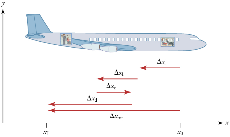
The smaller the time intervals considered in a motion, the more detailed the information. When we carry this process to its logical conclusion, we are left with an infinitesimally small interval. Over such an interval, the average velocity becomes the instantaneous velocity or the velocity at a specific instant. A car’s speedometer, for example, shows the magnitude (but not the direction) of the instantaneous velocity of the car. (Police give tickets based on instantaneous velocity, but when calculating how long it will take to get from one place to another on a road trip, you need to use average velocity.) Instantaneous velocity, [latex]v[/latex], is the average velocity at a specific instant in time (or over an infinitesimally small time interval).
Mathematically, finding instantaneous velocity, [latex]v[/latex], at a precise instant [latex]t[/latex] can involve taking a limit, a calculus operation beyond the scope of this text. However, under many circumstances, we can find precise values for instantaneous velocity without calculus. This is often done in biomechanics practice by measuring position (or displacement) over very small intervals of time, such as many hundreds of times per second. In many cases, average velocity will be lower than instantaneous velocity, for instance if the object is speeding up or slowing down during the measurement interval.
Speed
In everyday language, most people use the terms “speed” and “velocity” interchangeably. In biomechanics, however, they do not have the same meaning and they are distinct concepts. One major difference is that speed has no direction. Thus speed is a scalar. Just as we need to distinguish between instantaneous velocity and average velocity, we also need to distinguish between instantaneous speed and average speed.
Instantaneous speed is the magnitude of instantaneous velocity. For example, suppose the airplane passenger at one instant had an instantaneous velocity of −3.0 m/s (the minus meaning toward the rear of the plane). At that same time his instantaneous speed was 3.0 m/s. Or suppose that at one time during a shopping trip your instantaneous velocity is 40 km/h due north. Your instantaneous speed at that instant would be 40 km/h—the same magnitude but without a direction. Average speed, however, is very different from average velocity. Average speed is the distance traveled divided by elapsed time.
Average speed can be calculated by:
[latex]\bar {s} = \frac {d_{total}} {\Delta t}[/latex]
where
[latex]\bar{s}[/latex] is average speed, and
[latex]d_{total}[/latex] is total distance, and
[latex]\Delta t[/latex] is elapsed time
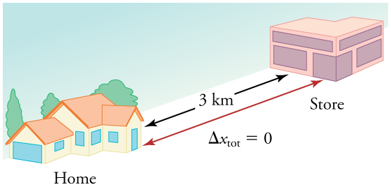
We have noted that distance traveled can be greater than the magnitude of displacement. So average speed can be greater than average velocity, which is displacement divided by time. For example, if you drive to a store and return home in half an hour, and your car’s odometer shows the total distance traveled was 6 km, then your average speed was 12 km/h. Your average velocity, however, was zero, because your displacement for the round trip is zero. (Displacement is change in position and, thus, is zero for a round trip.) Thus average speed is not simply the magnitude of average velocity.
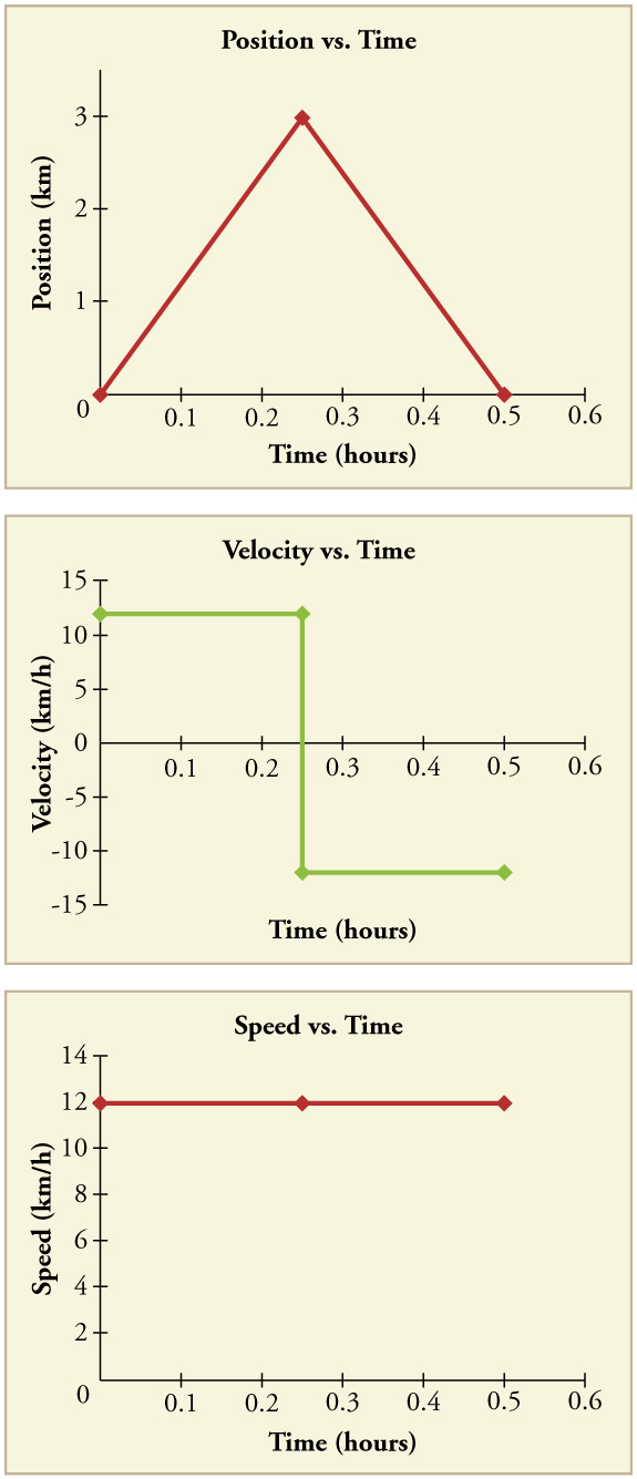
Graphing position, velocity and time
Another way of visualizing the motion of an object is to use a graph. A plot of position or of velocity as a function of time can be very useful. For example, for this trip to the store, the position, velocity, and speed-vs.-time graphs are displayed in Figure 2.11. (Note that these graphs depict a very simplified model of the trip. We are assuming that speed is constant during the trip, which is unrealistic given that we’ll probably stop at the store. But for simplicity’s sake, we will model it with no stops or changes in speed. We are also assuming that the route between the store and the house is a perfectly straight line.)
Making Connections: Take-Home Investigation—Getting a Sense of Speed
If you have spent much time driving, you probably have a good sense of speeds between about 10 and 70 miles per hour. But what are these in meters per second? What do we mean when we say that something is moving at 10 m/s? To get a better sense of what these values really mean, do some observations and calculations on your own:
- calculate typical car speeds in meters per second
- estimate jogging and walking speed by timing yourself; convert the measurements into both m/s and mi/h
- determine the speed of a sprinter, cyclist, and baseball (use estimates of distance and time)
Check your Understanding
A commuting cyclist travels from home to work, and back in 1 hour and 45 minutes. The distance between the two locations is approximately 13 miles. What is (a) the average velocity of the cyclist, and (b) the average speed of the cyclist in m/s?
(a) The average velocity of the cyclist is zero because [latex]{x}_{f}={x}_{0}[/latex]; the cyclist ends up at the same place they start.
(b) The average speed of the train is calculated below. Note that the cyclist travels 13 miles one way and 13 miles back, for a total distance of 26 miles.
