Chapter 1: Introduction
1.3 Accuracy and Precision
Authors: William Moebs, Samuel Ling, Jeff Sanny
Adapted by: Rob Pryce, Alix Blacklin
Learning Objectives
By the end of this section, you will be able to:
- Determine the correct number of significant figures for the result of a computation.
- Describe the relationship between the concepts of accuracy, precision, uncertainty, and discrepancy.
- Calculate the percent uncertainty of a measurement, given its value and its uncertainty.
- Determine the uncertainty of the result of a computation involving quantities with given uncertainties.
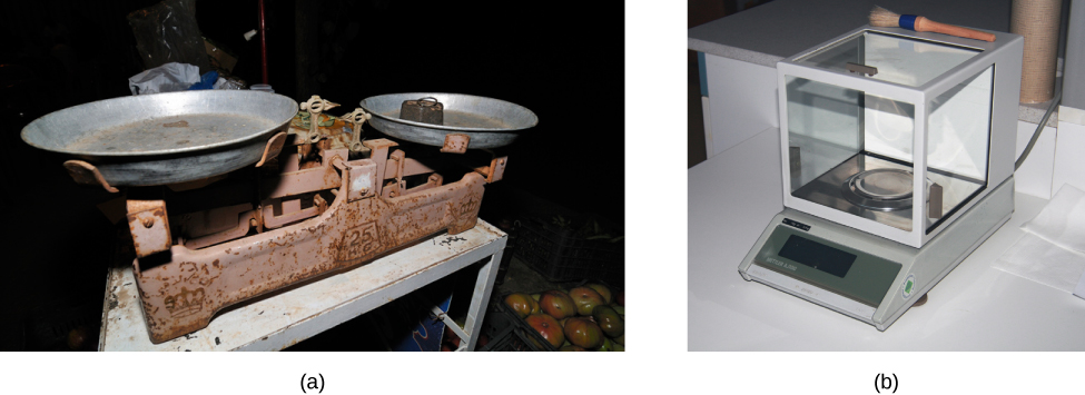
Figure 1.11 shows two instruments used to measure the mass of an object. The digital scale has mostly replaced the double-pan balance in most labs because it gives more accurate and precise measurements. But what exactly do we mean by accurate and precise? Aren’t they the same thing? In this section we examine in detail the process of making and reporting a measurement.
Accuracy and Precision of a Measurement
Biomechanics is based on observation and experiment—that is, on measurements. There are specific parameters used to describe measurements:
Accuracy is how close a measurement is to the correct value for that measurement. For example, let us say that you are measuring the distance of a running tack. The international standard for running track length provided by the IAAF specifies the inside lane of the track should be 400m (measured 20-30 centimetres from the inside border) Assuming the track is known to be exactly 400.0m, you measure the length of the track three times and obtain the following measurements: 401.4m, 400.9m and 399.4m. These measurements are quite accurate because they are very close to the correct value of 400.0m. In contrast, if you had obtained measurements of 385.1, 415.3, and 430.2m, your measurements would not be very accurate. Notice that the number of decimal places used doesn’t necessarily relate to accuracy – you could have obtained a measurement of 430.23156m, which would have been similarly inaccurate .
The precision of a measurement system refers to how close the agreement is between repeated measurements (which are repeated under the same conditions). For the measurements of the running track above the precision of the measurements refers to the spread of the measured values. One way to analyze the precision of the measurements would be to determine the range, or difference, between the lowest and the highest measured values. In that case, the lowest value was 399.4m and the highest value was 401.4m. Therefore the range is 401.4m – 399.4m = 2.0m, indicating the measured values deviated from each other by at most 2.0m
Regardless of which method is used, they all show that the measurements were relatively precise because they did not vary too much in value. However, if the measured values had been 401.4m, 399.4m and 430.2m, then the measurements would not be very precise because there would be significant variation from one measurement to another.
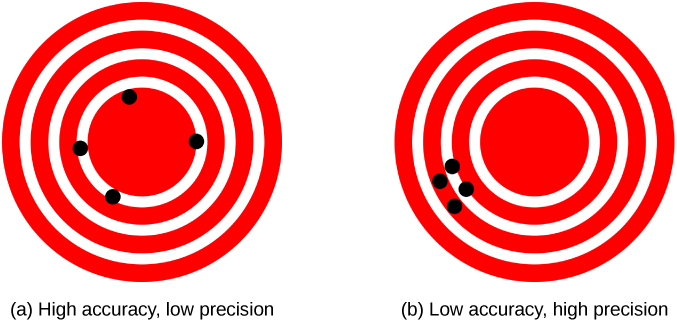
The measurements in the example above are both accurate and precise, but in some cases, measurements are accurate but not precise, or they are precise but not accurate. Let us consider an example of a GPS system that is attempting to locate the position of an athlete on a soccer field. Think of the actual position of the athlete as existing at the center of a bull’s-eye target, and think of each GPS attempt to locate the restaurant as a black dot. (GPS positions will always have some error due to factors such as the number of satellites connected or obstructions from nearby buildings or trees).
In Figure 1.12 a) , you can see that the GPS measurements are spread out far apart from each other, but they are all relatively close to the actual location of the athlete at the center of the target. This indicates a low precision, high accuracy measuring system (the error in this GPS system is likely random). However, in Figure 1.12 b), the GPS measurements are concentrated quite closely to one another, but they are far away from the actual location. This indicates a high precision, low accuracy measuring system (there might be a systematic error in this GPS system).
Accuracy, Precision, Uncertainty, and Discrepancy
The precision of a measuring system is related to the uncertainty in the measurements whereas the accuracy is related to the discrepancy from the actual known value or accepted reference value (if unknown). Uncertainty is a quantitative measure of how much your measured values deviate from one another. Discrepancy (or “measurement error”) is the difference between the measured value and a given standard or expected value. If the measurements are not very precise, then the uncertainty of the values is high. If the measurements are not very accurate, then the discrepancy of the values is high.
One way to better understand (or estimate) uncertainty and discrepancy is to take more than one measurement (like the 3 measurements of the same running track above). Such multiple measurements are also important when measuring more than one object, person or event. However, these multiple measurements present a challenge – how do we report them? Do we report all 3 measures of the running track above? The ‘best’ one? The ‘worst’ one? These are important decisions in biomechanics.
It turns out that only very rarely will we report every single measurement or our ‘raw data’ (e.g., all 3 measures of the running track), instead we’ll want to simplify and interpret these numbers for our audience.
Accuracy and Discrepancy
One of the most obvious ways to do this to report the average, or arithmetic mean, of the measures. This is simply the sum of all the measures (401.4 + 400.9 + 399.4) divided by the number of measurements (3). For the example above, this is equal to 400.6m. We could then estimate the discrepancy by subtracting the known distance from our average (400.6m – 400.0m = 0.6m), which provides a quantitative measure of accuracy. This mean value also gives an indication of the ‘central tendency’ (or approximate ‘middle’) of our measurements. Sometimes you may encounter other measures of central tendency, such as median or mode, depending on the characteristics of your data (for more on that, make sure you pay attention in your introductory statistics course). In biomechanics we most often deal with data that is best represented by the arithmetic mean.
Precision and Uncertainty
Next, we need a way to report the uncertainty, or variability, in the measurements. There are many different methods of calculating uncertainty, each of which is appropriate to different situations. One method is to report the uncertainty based on the range, (that is, the biggest less the smallest). Often this is done by taking half of the range of the measured values. For the running track above, the range was 2.0m, and therefore half of the range is 2.0m / 2 = 1.0m. Then we would say the distance of the track is 400.6m. plus or minus 1.0m. The uncertainty in a measurement is often denoted using the lowercase Greek letter delta, δ. So, for a measurement, A, this would be recorded as , A ± δA. Returning to our track example, the measured distance of the track could be expressed as 400.6 ± 1.0 m. Since the discrepancy of 0.6m. is less than the uncertainty of 1.0m, we might say the measured value (400.6m) agrees with the accepted reference value (400.0m) to within experimental uncertainty (+/-1.0m).
However, in biomechanics it is more common to report uncertainty or variation using other methods. This is especially true when dealing with multiple measures on different people, objects or events. Interestingly, these methods also report an average, but in this case it’s an average of the uncertainty in each measure.
1. For instance, we could simply subtract the mean (400.6m) from each measurement to obtain the uncertainty for each measure:
-
- 401.4 – 400.6 = 0.8
- 400.9 – 400.6 = 0.3
- 399.4 – 400.6 = -1.2
and then take the average of those numbers: (0.8 + 0.3 -1.2) / 3 = -0.03m.
However, you’ll notice a problem here: since the measurements were both above and below the mean this yielded both positive (0.8 and 0.3) and negative numbers (-1.2) for the uncertainty of each measurement. When those numbers were added together to calculate the average uncertainty across all measures, it reduced the actual uncertainty. That is, -0.03m sounds like a very precise measure, when in fact all of the measures varied from the mean by at least 10 times that amount. So, to get around this issue, scientists have other options when reporting uncertainty or variation.
2. Report the mean absolute difference, which is calculated by taking the absolute value of the uncertainties for each measure, and then reporting the average of those. The absolute value is merely the non-negative value of a number and reflects its overall magnitude (or size), without reference to whether it is + or -. Expressing uncertainty as the mean absolute difference yields 0.8m, which better reflects the variation. We could state this in plain language by saying “the measurements varied by an average of 0.8m”.
3. Report the variance, which is the average of the squares of the difference from the mean. This sounds more complicated, but has the same effect as the mean absolute difference. That is, the square of a negative number is always positive. Reporting variance is actually the more common approach, particularly if the biomechanist is going to use statistics to analyze their data. The variance of the measurements is: 0.7 m.
4. The most common way of reporting uncertainty in biomechanics is by the standard deviation, which is just the square root of the variance. The standard deviation of the measurements is: 0.9m.
Regardless of the method used, all of these numbers communicate information about the uncertainty or variation in the measurements. Which approach you use will depend upon your audience and intended purpose – for communicating with other scientists and/or when using statistics, we almost always report standard deviation. However, when communicating with non-scientific knowledge users or the lay public it might be more intuitive to report the range or mean absolute difference.
Factors affecting uncertainty
Some factors that contribute to uncertainty include:
- Limitations of the measuring device
- The skill of the person taking the measurement
- Irregularities in the object being measured
- Any other factors that affect the outcome (highly dependent on the situation)
In our example, factors contributing to the uncertainty could be the smallest division on the measuring device we used. For example, perhaps you measured the track with a suveyor’s wheel (or hodometer) and it only reports to the nearest 10cm (or 0.1 of a meter). Or maybe the device was worn out and didn’t register every revolution, or perhaps you walked in a slightly wobbly path, or didn’t mark the start/end of the track precisely, or forgot to reset the counter to zero before starting. All of these factors could have contributed to uncertainty. At any rate, the uncertainty in a measurement must be calculated to quantify its precision. If a reference value is known (which is somewhat rare in biomechanics), it makes sense to calculate the discrepancy as well to quantify its accuracy.
MAKING CONNECTIONS: REAL-WORLD CONNECTIONS – On the podium or not?
Uncertainty is a critical piece of information in biomechanics.
Imagine you are responsible for measuring results of the shot put at the most recent Olympics games, which were held in Beijing in 2020. In shot put, the distance thrown is measured from the inside of the launching circle to the nearest mark made in the ground by the falling shot, often using a measuring tape.
In 2020 Olympics, the gold, silver and bronze medals in shotput went to Lijiao Gong (China), Raven Saunders (US) and Valerie Adams (NZ) with distances of 20.58, 19.79 and 19.62m, respectively. Auriol Dongmo (PT) also had an exceptional throw of 19.57m.
What if the uncertainty of your measurements was +/- 0.06 m? For example, due to measurement technique, alignment, stretch in the tape, etc.
In that case, the ‘true’ distance of Auriol’s throw could be anywhere from 19.51 to 19.63, which would overlap with Valerie’s throw of 19.62m (which would have its own uncertainty of 19.56 to 19.68m). So, a measuring technique with an uncertainty of 0.06m would be useless for events where the difference between positions are less than that, in this case measured to the nearest 0.01m (a value smaller than the uncertainty in the measurement).
Percent uncertainty
Another method of expressing uncertainty is as a percent of the measured value - in other words as a relative uncertainty. One reason to express uncertainty as a percentage is if the audience is unfamiliar with the scale or reference points you’re using. For instance, is the uncertainty (mean absolute difference) of 0.8m in the example above large or small? Representing as a percentage can help give a better sense of the size of the uncertainty.
The percent uncertainty can be obtained by dividing the uncertainty (δA) by the average (A) and multiplying by 100:
[latex]\text{Percent uncertainty}=\frac{\delta A}{A}\,×\,100%.[/latex]
We can see that as a percentage, the uncertainty in the measurements of the track above is quite small: 0.8/400.6 x 100 = 0.2%. By contrast, an absolute uncertainty of 0.8m would be very large for measuring of human heights (which range from ~1.0m to 2.4m).
Another use for percentages is when reporting differences between groups or changes over time – here, percentages can help give the reader a better sense of the scale of the change. To calculate the percent change, divide the change by the original value and multiple by 100.
Example 1.1
Calculating Percent Uncertainty: Golf ball regulations
PGA regulations state that golf balls can have a mass of no more than 45.9g. Let’s say we purchase 6 golf balls from a single manufacturer and we obtain the following measurements:
Table 1.3 Variation in mass of 6 golf balls of the same model and manufacturer.
| Ball | Mass (g) |
| 1 | 45.5 |
| 2 | 44.9 |
| 3 | 46.6 |
| 4 | 45.8 |
| 5 | 44.3 |
| 6 | 44.2 |
We then determine the average mass of the balls is 45.2, with a range of ± 2.4g (46.6 – 44.2 = 2.4). Using the simple approach to uncertainty of half the range, we could state the results of the measurements as 45.2±1.2g. What are these results using percent uncertainty?
Strategy
First, observe that the average value of the golf balls’ mass, A, is 45.2g. The uncertainty in this value, [latex]\delta A,[/latex] is 1.2g. We can use the following equation to determine the percent uncertainty of the weight:
[latex]\text{Percent uncertainty}=\frac{\delta A}{A} \times 100[/latex]
Solution
Substitute the values into the equation:
[latex]\text{Percent uncertainty} = \frac{\delta {A}}{A} \times 100 = \frac{1.2 \text{lb}}{45.2 \text{lb}} \times 100 = 2.7\text{%} \text { or ~3%.}[/latex]
Discussion
We can conclude the average mass of the golf balls is 45.2g±2.7%.
Check your Understanding
- Given the uncertainty in measurements of the golf balls above, would you be confident using them in a PGA tournament? Why or why not?
- Assume you measured the track above a 4th time, and obtained a measurement of 408.6m, in addition to the first three measures above (401.4m, 399.4m, 400.9m). Can you calculate the average, range, mean absolute difference, variance and standard deviation of those measurements? What do these numbers say about the accuracy and precision of your measures?
Uncertainties when doing calculations
Occasionally we will encounter situations where we must do a calculation involving multiple values, each with their own uncertainty. For example, velocity is calculated from measurements of displacement and time. What will the uncertainty be in velocity?
When we are performing calculations that involve multiplication or division, then the method of adding percents can be used. This method states the percent uncertainty in a quantity calculated by multiplication or division is the sum of the percent uncertainties in the items used to make the calculation. For example, if the displacement is 7.7m with an uncertainty of 2% and the time was 3.5 seconds with an uncertainty of 1%, then the velocity is 2.2 m/s and has an uncertainty of 3%. (the percentage uncertainty can be converted to units of m/s via 2.2 * .03 = 0.6 m/s)
Significant Figures and precision
An important factor in the precision of measurements involves the precision of the measuring tool itself. That is, precision is related to both the tool as well as other factors such as operator experience (see ‘Factors affecting uncertainty’ above). In general, a precise measuring tool is one that can measure values in small increments. For example, a standard weigh scale can measure to the nearest 100 grams, whereas a research-grade force plate can measure to the nearest 1g or less. (note: for convenience, units of grams are provided here, however the output of force plates – and other weigh scales – is best expressed in units of Newton’s). The force plate is a more precise measuring tool because it can measure extremely small differences. The more precise the measuring tool, the more precise the measurements.
When we express measured values, we can only list as many digits as we measured initially with our measuring tool. For example, if we use a standard weigh scale (which measures to the nearest 100g) to measure body mass, we may report our measurement as 84.1 kg. We can’t express this value as 84.12 kg because our measuring tool is not precise enough to measure a hundredth of a kilogram.
Using the method of significant figures, the rule is that the last digit written down in a measurement is the first digit with some uncertainty. To determine the number of significant digits in a value, start with the first measured value at the left and count the number of digits through the last digit written on the right. For example, the measured value 84.1 kg has three digits, or three significant figures. Significant figures indicate the precision of the measuring tool used to measure a value.
Zeros
Special consideration is given to zeros when counting significant figures. For example, the zeros in in 0.053 kg are not significant because they are just placeholders that locate the decimal point. There are two significant figures in 0.053 kg (‘5’ and ‘3’). It could also be written in units of grams as 53 g, or in scientific notation as 5.3 x 10⁻² kg – all convey the same precision and have the same number of significant figures.
Conversely, the zeros in 10.053 kg are not placeholders; they are significant. This number has five significant figures.
Finally, the zeros in 1300 grams may or may not be significant, depending on the style of writing numbers and properties of the measurement. They could mean the number is known to the last digit (nearest gram) or they could be placeholders (nearest 100 grams). So 1300 grams could have two, three, or four significant figures. To avoid this ambiguity, biomechanists often write numbers like 1300 in scientific notation as 1.3 x 10^3, 1.30 x 10^3, or 1.3 x 10^3, depending on whether it has two, three, or four significant figures. Zeros are significant except when they serve only as placeholders.
Significant figures in calculations
When combining measurements with different degrees of precision, the number of significant digits in the final answer can be no greater than the number of significant digits in the least-precise measured value. There are two different rules, one for multiplication and division and the other for addition and subtraction.
1. For multiplication and division, the result should have the same number of significant figures as the quantity with the least number of significant figures entering into the calculation.
Using the velocity example above, both the distance (7.7 m) and time (3.5 seconds) have two significant figures, so the answer should be written as 2.2 m/s.That calculation is straightforward because the answer naturally has the same number of significant figures. What would happen if the time was changed to 2.0 seconds? First, it would be reasonable to assume that 2.0 has two significant figures, since the writer when through the trouble of writing ‘2.0’ vs 2. However, when we calculate velocity, we get:7.7 m / 2.0 s = 3.85 m/sBut because the displacement and time both have two significant figures this should be written as 3.9 m/s.Similarly, if the time was written as 2 seconds (only 1 significant digit), then the velocity would be written as 4 m/s to correspond to the least number of significant figures.
2. For addition and subtraction, the answer can contain no more decimal places than the least-precise measurement.
Suppose you are monitoring your change in body mass at the start, middle and end of a 10-week weight training program. At the start of the program, you measured your body mass at your nearby gym, which was 72.1 kg, as measured measured on a scale with precision 0.1 kg. At 5-weeks you measure your body mass at 73.06 kg on your university’s laboratory scale, which has a precision of 0.01 kg. Lastly, at 10-weeks you weigh yourself at home on a simple bathroom scale, which measures to the nearest 1kg, and find a value of 74 kg. How much did your body mass change over the 10-week program? The answer is found by simple addition and subtraction:74 – 72.1 = 1.9 kgNext, we identify the least-precise measurement: 74 kg. This measurement is expressed to the nearest 1kg, so our final answer must also be expressed to the nearest 1 kg. Thus, the answer is rounded to 2 kg.What about the change in body mass from the start to 5-week point? These are more precise measures than the bathroom scale, and so the answer can be expressed to the nearest 0.1 kg (having the same number of decimal places as the least precise measurement).
Significant figures in this text
In this text, most numbers are assumed to have three significant figures. Furthermore, consistent numbers of significant figures are used in all worked examples. An answer given to three digits is based on input good to at least three digits, for example. If the input has fewer significant figures, the answer will also have fewer significant figures. Care is also taken that the number of significant figures is reasonable for the situation posed. Also, if a number is exact, such as the two in the formula for the circumference of a circle, C = 2πr, it does not affect the number of significant figures in a calculation. Likewise, conversion factors such as 100 cm/1 m are considered exact and do not affect the number of significant figures in a calculation.
