Main Body
2 Making Sense of Large Image Datasets
Ryleigh Bruce; Mitchell Constable; and Zhenggang Li
This section provides a brief overview of methods for exploring and automating the visualization and organization of large image datasets.
One challenge in making sense of large collections of images is understanding which questions to ask. It can be helpful to get an overview of the dataset, visualizing its contents to understand the overall distribution of images. It can also be helpful to filter the dataset, visualizing subsets of the entire dataset to get an understanding of variation and local characteristics. In the case of the animals dataset, images can be filtered by time of day, day and night, time of year, location, and species.
Filtering and search
Filtering images
If image filenames contain information about the image contents, it becomes easy to sort and filter the images using these details. Image filenames in the Wild Winnipeg dataset are organized in the format ‘xxx’ and contain information about the date the image was captured, the camera number, and animal species present in the image. The information in the filename can be used to sort the images or filter them into subsets based on the information provided. This can be accomplished with Python scripts, as described in the Image Filter Jupyter Notebook, and filters can also be applied using the search function in the MacOS, Linux or Windows file browser.
Manual Review of Random Selections
When analyzing large image sets, it can be helpful to review a sample of images selected randomly, as a method for understanding the content and variation contained within the dataset (figure 2.1). This process can be automated using a Python script that randomly selects and moves the desired number of images and displays them. The scripts in the Random Manual Review Jupyter Notebook were used by the Wild Winnipeg team to create data subsets to test YOLO model training.
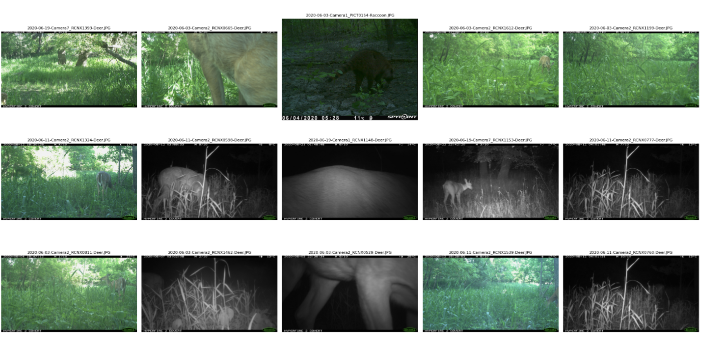
Figure 2.1: Visual output of the Random Manual Review Jupyter Notebook. A sample of the selected images are displayed along with their file names to confirm script functionality.
Selecting Random Interactive Images for Review
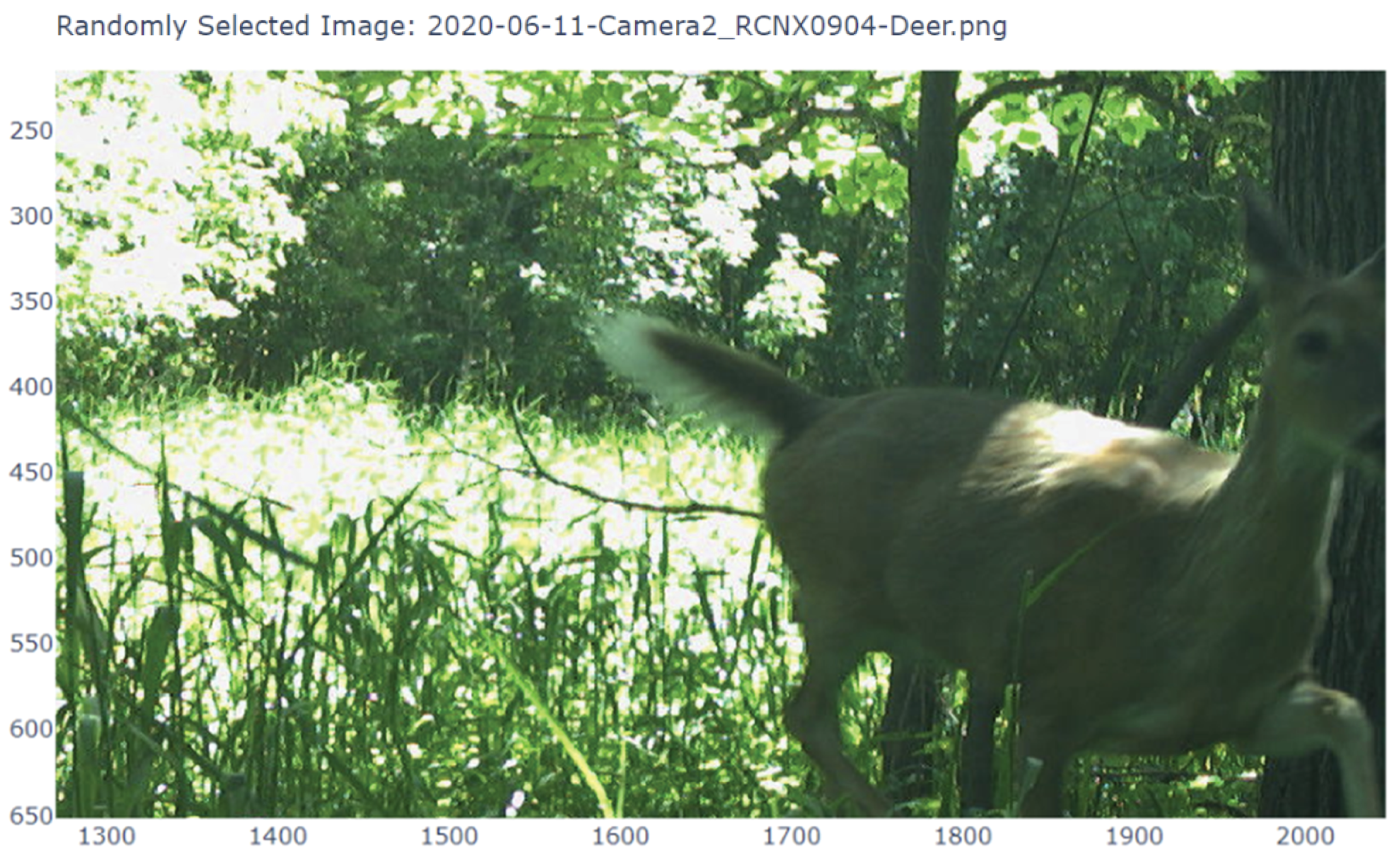
This workflow selects random images and displays them in the terminal space to be reviewed, as an alternative to manually selecting images to examine in closer detail (figure 2.2). The Python script presented in the Random Manual Review Jupyter Notebook displays the randomly selected image and allows the user to interact with it by zooming in on specific regions. This feature is particularly useful when attempting to analyze finer details of an image set or when reviewing images analyzed by a machine learning model for accuracy.
Visualizing Image Information
This section provides a brief overview of the process of using AI-generated Python code to extract and visualize data from large sets of images.
Creating an Image Grid
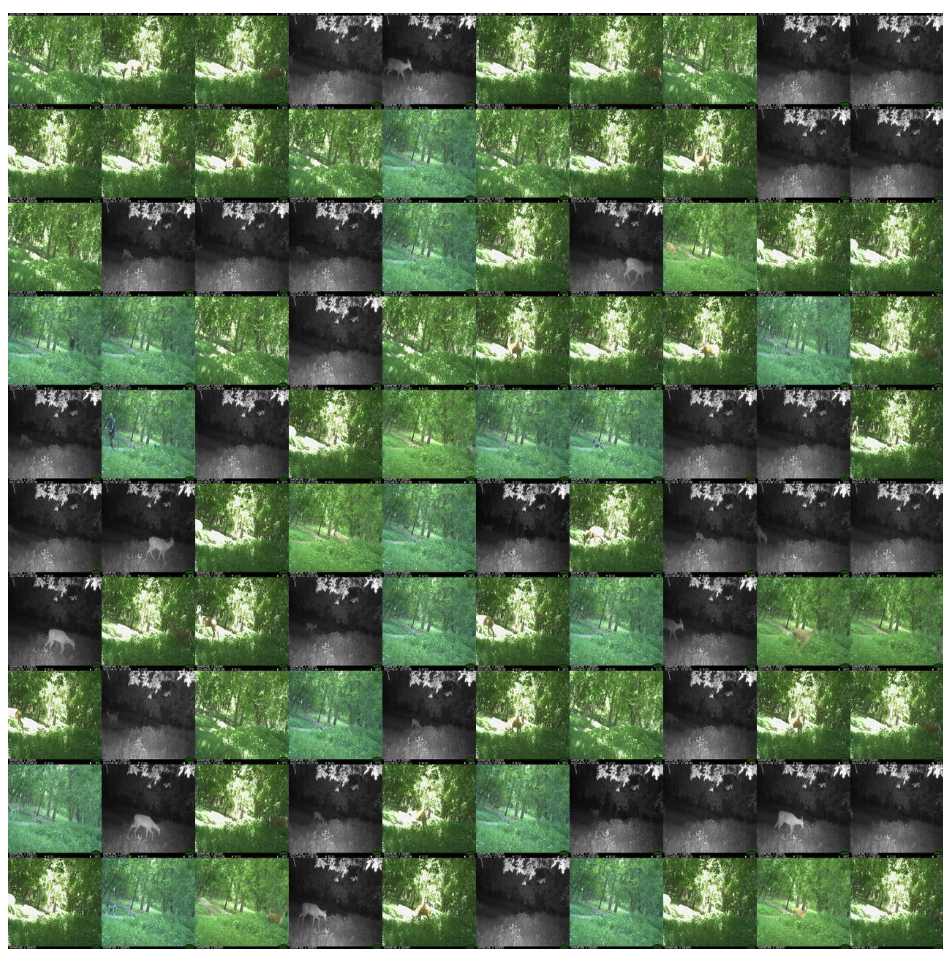
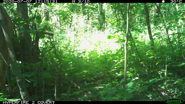
One quick method for finding patterns in an image dataset is to create an image grid, a collection of miniature images that facilitates the visual identification of patterns across the dataset. For example, in figure 2.3, there are visible patterns in the image grid related to the weather (intensity of direct sunlight), vegetation on the site, as well as the day versus night. A grid with thousands of small images can be used to analyze general patterns that do not require a detailed view of each individual image. Alternately, a series of grids with fewer, larger images can be used to inspect for more subtle visual patterns that require a detailed view of each image. Both types of image grid can be generated using the script in the 100 Image-grid Jupyter Notebook.
Generating Visualizations from Extracted Data
Image datasets are often accompanied by a file containing associated metadata, often including details regarding image date, camera location, and any other relevant details. The Wild Winnipeg project dataset includes an Excel file that for each image logs the information associated with the image. Categories of data captured by the camera at the time of capturing an image include date, time, temperature, moon phase, image quality, and ambient light. Additional categories of information that were added manually for each image include the animal species present in the image, species count, the activity the animals are engaged in, and animal gender. This detailed file allows the user to generate a series of charts and graphs visualizing the relationships between each category.
A variety of visualization techniques can be generated using Python scripts (figure 2.4). Tutorials on generating bar graphs, line graphs, scatter plots, tree maps, and other custom visualizations can be found in the Tree Map (figure 2.5), Sightings Bar Graph, and Matplotlib Visualization Jupyter Notebooks.
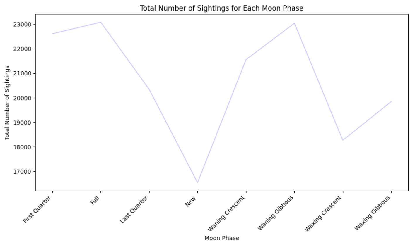
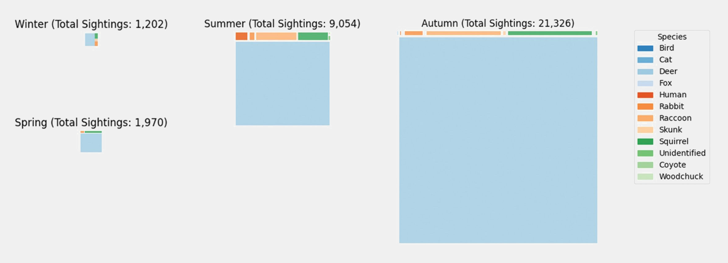
Figure 2.5: An example of a more complex visualization that can be generated using image metadata. This is a series of tree maps visualizing the volume of sightings across seasons for each animal species, with the relative size of each individual tree map demonstrating the comparative volume of overall sightings across the seasons.
Close Encounters Data
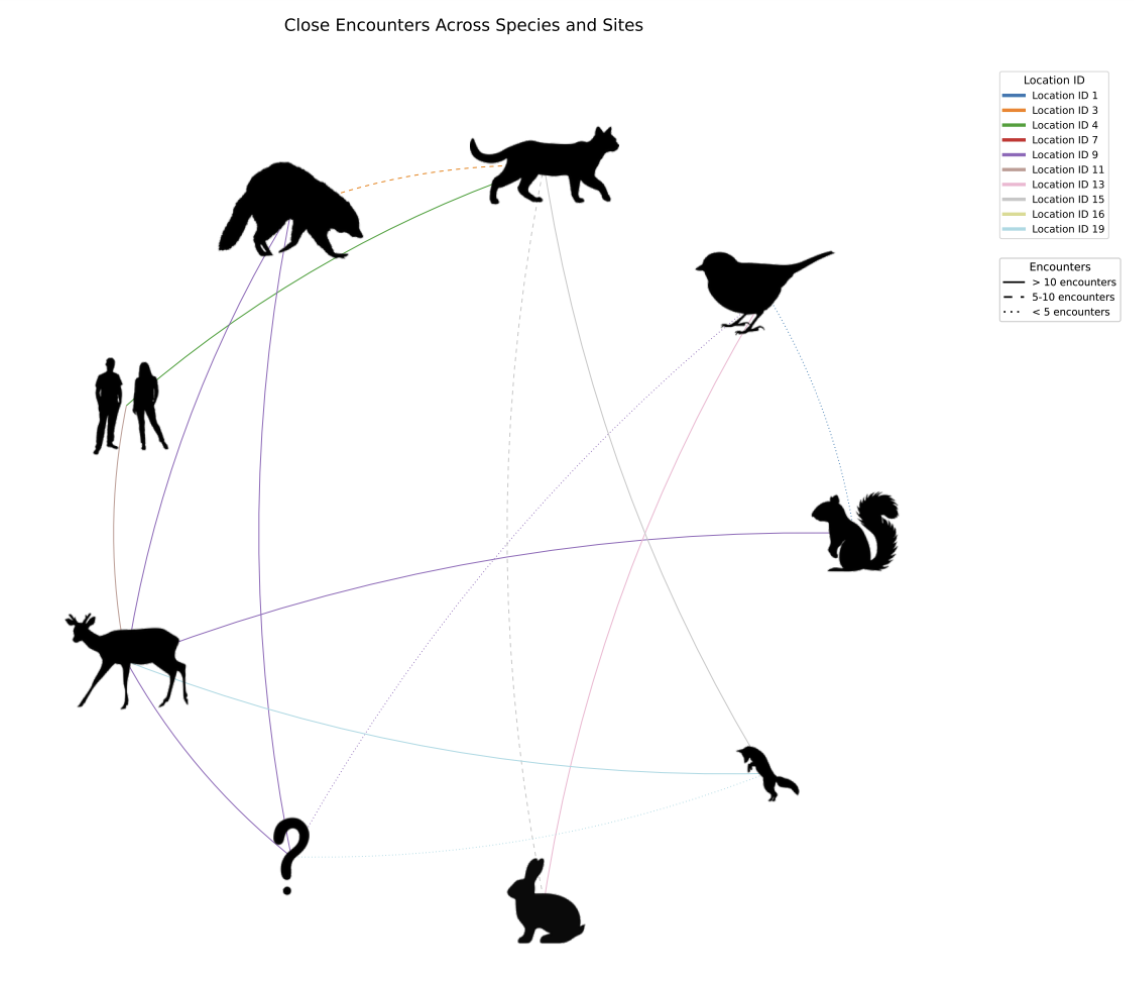
One opportunity provided by the comprehensive metadata from the Wild Winnipeg project is the chance to examine relationships between different animals, as well as relationships between suburban wildlife and humans. The specific information analyzed by the team is close encounter data. A close encounter is defined here as two or more mammals observed by a camera at the same location on the same day within ten minutes of each other. Any observations meeting these criteria that occur within one minute of each other are classified as a ‘sequence,’ which counts as a single observation of the identified mammal. This information has been analyzed in the form of network visualization graphs (figure 2.6).
These graphs represent each class of animal as a node, connected by a series of edges whose line type and colour represent the volume of close encounters along with the location of the close encounter, respectively.
The intent of analyzing this data is to reflect on the significance of wildlife in an urban setting and how ephemeral wildlife sightings shape urban experiences. Additionally, it is critical to understand how these encounters shape the activity of mammals that live within urban woodlands to preserve these spaces and promote awareness of how human spaces impact the existence of other living things. Information on how to generate a network graph using Python code can be found in the Close Encounters Jupyter Notebook.
Fine-tuning the YOLOv8 Object Localization Model
This section provides a brief overview of the process of fine-tuning the classification model on a specialized dataset to increase its performance on identifying objects within an image set via bounding box annotation.
Design Applications
The YOLOv8 model is particularly useful in the design realm due to its accessibility to designers with little to no prior coding experience. The pre-trained model has excellent general knowledge that can be used to extract information from large image sets. It is simple to train with powerful results and offers a variety of image analysis techniques.
A fine-tuned YOLOv8 model has exciting potential for applications throughout the design process. It is particularly useful for extracting key information efficiently and accurately from large image sets collected during stages of design, such as site analysis. This information can be used to analyze phenomena relevant to design that are otherwise difficult to investigate, such as how urban activity influences urban wildlife or how infrastructure shapes day-to-day activity and experiences at the human scale.
Model Overview
The YOLO (You Only Look Once) object detection model was originally developed by Joseph Redmon and Ali Farhadi at the University of Washington in 2015. YOLOv8 is the latest version of the model at the creation of this document and provides features such as object detection, segmentation, pose estimation, object tracking, and image classification.[1] The YOLO model has been trained on vast image datasets, such as the COCO (Common Objects in Context) dataset, which comprises over 330 000 images and 80 object classes.[2]
The YOLO model is innovative due to its single-shot detection approach that performs object detection by processing an entire image simultaneously, rather than using traditional two-stage detection methods that employ region proposal networks and sliding window techniques for object localization. This unified architecture in the YOLO model drastically reduces the required inference time and computational resources for performing real-time object detection tasks. Additionally, the YOLOv8 model employs data augmentation techniques such as geometric transformations (rotation, horizontal flipping) and photometric distortions to enhance model generalization and mitigate overfitting during training.[3]
What is Fine-tuning?
When training the YOLO model to increase its performance at a specific task, one can either train it entirely from scratch or modify an existing model. The latter is done by training the existing model on a smaller, more specialized dataset. Training a model entirely from scratch, particularly a YOLO model, requires a large dataset and extensive computational resources, which is not always practical. Fine-tuning a model involves training a model with existing weights on a much smaller dataset, requiring less time and computational resources.
To fine-tune a YOLO model on a custom dataset (figure 2.7), it is critical to ensure that the image and label files are properly formatted. When fine-tuning a model on an object localization dataset, the training and validation images should be visually clear of bounding boxes, but the label files (.json files) should include the class of the identified object along with the bounding box coordinates. Having this information provides a ground truth for the model to learn from, rather than allowing it to simply guess where the subject is within the image.
Overall, fine-tuning the YOLO model is an excellent way to take a model trained on very general data and increase its ability to perform a task within a specific context. In our project, that context is the study of large mammals in the suburban woodlands of Winnipeg.
Downloading a Pre-made Dataset: Huggingface, Kaggle, and FiftyOne Data Zoo
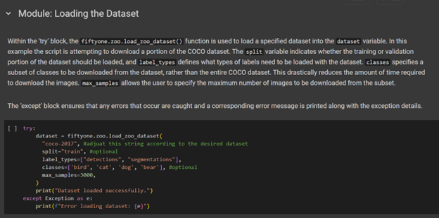
If one does not have access to enough data to create an entirely custom dataset to fine-tune a model, there are several platforms that host a wealth of high-quality open-source datasets. Hugging Face hosts models and data sets specifically targeted for AI training. Kaggle hosts models, data sets, competitions, courses, and discussion platforms targeted towards AI training and machine learning.
The FiftyOne Data Zoo is a particularly useful platform as it allows you to download partial datasets directly within your coding environment. Further instructions on how to do this can be found in the Data-Prep Jupyter Notebook. This notebook covers steps such as downloading an open-source dataset, splitting a dataset, and creating a YAML file. The latter two topics will be explored in greater detail later in this guide.
Creating a Custom Dataset
Curating the Dataset
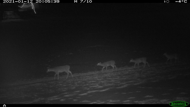
When fine-tuning an object localization model, it is critical to have a varied dataset to increase the model’s generalizability (figure 2.8). The YOLOv8 model has built-in data augmentation features that are especially useful for varying the dataset during training. These data augmentation techniques include rotating images, mirroring them, increasing visual noise, and modifying image hue and saturation. Incorporating these features into the fine-tuning script also aids in increasing the model’s prediction accuracy.
In addition to having a varied dataset, it is important to have a dataset that represents each of its classes relatively equally (figure 2.9). Training a model on an unbalanced dataset increases the likelihood of producing an inherently biased model. One technique for addressing an unbalanced dataset is to combine your custom dataset with portions of a pre-existing dataset containing a higher volume of the same or similar classes. The FiftyOne Data Zoo’s ability to download specific classes and portions of open-source datasets is particularly useful for this purpose.
Creating Label Files
Each label file should follow the same naming convention as its image counterpart, with the addition of the .txt suffix. This means that an image called Camera1_2021-05-21_Raccoon_123 would have a corresponding label file named Camera1_2021-05-21_Raccoon_123.txt (or the suffix .json, depending on the file format). If this naming convention is not followed, the model will be unable to recognize the corresponding label files during the fine-tuning process.
Label files for fine-tuning the YOLO model for the object localization task are typically in .txt or .json format. Each line within the file represents a single bounding box indicating the location of an object, and multiple object predictions within a single image will result in multiple lines of text within the label file.
Each label file contains the class number of the predicted object, followed by the coordinates of the corresponding bounding box. For example, within the custom Wild Winnipeg dataset, the raccoon is the seventh class. Thus, a label file for a raccoon prediction may contain: 7 0.493850385 0.404802841 0.485723947 0.954762948. Note that YOLO training label files will only contain positive values.
When creating a custom dataset, there are several software options available for label file generation, all of which require manual bounding box labelling. The program used for the creation of the Wild Winnipeg custom dataset was Labelme, which can be installed through the Windows Command Prompt.
Splitting the Dataset
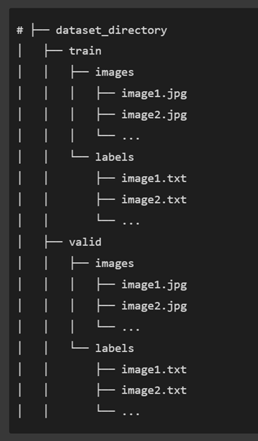
When fine-tuning an object localization model, the dataset must be split into training and validation folders (figure 2.10). This can be done manually or, much more efficiently, with a Python script such as the one found in the Data-Prep Jupyter Notebook. The most common training/validation split is 0.2, meaning 80% of the dataset is used for training and the remaining 20% for validation.
When splitting the dataset, a specific directory organization must be followed. The structure for the object localization model training is visualized in figure 3.10, but it consists of separate training and validation folders within a main directory, with each of these subfolders containing separate directories for image files and their accompanying label files.
When using an automated script to split the dataset, it is critical to ensure the script is modified appropriately to handle different file types and directory structure requirements.
The YAML File
The YAML file is the legend provided to the YOLO model to understand the information within the label files (figure 2.11). It tells the model where to locate the training and validation files, the total number of classes, and the class names in string format.
When listing the classes in the YAML file, the first class is class 0 unless otherwise specified. This means that a YAML file with the classes listed in the following format [‘rabbit’, ‘deer’, ‘fox’, ‘dog’] contains four classes, with ‘rabbit’ being class 0.
However, if each class is explicitly assigned a value starting at one in the following format:
Order:
1: rabbit
2: deer
3: fox
4: dog
Then there are four classes, with ‘rabbit’ being class 1.

Fine-tuning YOLOv8 for Object Localization Tasks
Fine-tuning the YOLOv8 model for increased performance at the object localization task requires extensive time and computational resources. A training script for 100 epochs with the minimum batch size took twelve hours alone on a remote desktop. The script used for fine-tuning our model can be found in the YOLO Fine-tuning Jupyter Notebook.
Once the fine-tuning script has successfully run, a weights file, or .pt file, is generated. This file can then be used to implement the trained model. The script will also produce performance metrics for each class it has been trained on, allowing the user to analyze its current performance and adjust the number of epochs and the batch size accordingly.
Notes
- Ultralytics. "Ultralytics YOLO Docs." Accessed July 24, 2024. https://docs.ultralytics.com/. ↵
- COCO. "COCO - Common Objects in Context." Accessed July 24, 2024. https://cocodataset.org/#home. ↵
- Torres, Jane. "YOLOv8 Architecture: A Deep Dive into its Architecture." YOLOv8. Accessed July 24, 2024, https://yolov8.org/yolov8-architecture/. ↵
A programming language used throughout the documents for creating scripts that utilize machine learning models, automate image processing tasks, generate prompts for Stable Diffusion, and implement various data analysis and visualization functions in the context of wildlife image classification research.
Two or more mammals observed by a camera at the same location on the same day within ten minutes of each other. Any observations meeting these criteria but that occur within one minute of each other are classified as a ‘sequence,’ which counts as a single observation of the identified mammal.
An object detection model that performs detection by processing an entire image simultaneously, rather than using traditional two-stage detection methods, making it faster and more efficient for real-time applications.
A computer vision task that involves identifying and locating objects within images, typically using bounding boxes to indicate object positions.
Segmentation is a method of object identification provided by the YOLOv8 model. It involves analyzing every pixel within a given image and predicting which pixels belong to a known class. These pixels are then identified with a semi-opaque coloured mask, and this model frames the mask with a bounding box that states the predicted class and confidence score in decimal format. Segmentation mask labels follow a similar format to bounding box labels, however, they contain the coordinates of each pixel that forms the edge of the mask.
Pose estimation is an image analysis technique offered by the YOLOv8 model. It identifies human postures within an image by identifying key points with coloured nodes and connecting them to create a wire frame figure. Although the pre-trained model only offers this technique to analyze human postures, several open-source datasets exist to fine-tune the model to approximate various animal postures.
The simplest image analysis technique offered by YOLOv8, image classification involves identifying what class the objects within a given image belong to and provides the class name and confidence score. This technique does not identify the location of the predicted objects within a given image.
Occurs when the model is trained with too many epochs on a dataset, resulting in inaccurately high performance metrics and inhibiting the model’s ability to generalize on other image sets. This can be avoided by ceasing model training when performance metrics plateau.
Bounding boxes are a method of object localization provided by the YOLOv8 model. They are intended to tightly frame the identified object, and it is best practice to minimize the amount of excess space between the subject and the bounding box. When creating bounding boxes by hand to obtain ground truth for training models, the coordinates of the bounding box will typically be generated in a .json file containing the coordinates of the top-left and bottom-right corners. When the bounding boxes are annotated by a trained model, confidence scores are often labeled with the box in decimal format.
A configuration file that serves as a legend for machine learning models, telling the model where to locate training and validation files, the total number of classes, and class names in string format.
A built-in feature of YOLOv8 model training that involves manipulating aspects of the training images to increase model accuracy and generalizability. This is done by modifying image saturation, hue, orientation, or noise levels, amongst other characteristics.
The process of teaching a machine learning algorithm to make accurate predictions by feeding it labeled data examples, allowing the model to learn patterns and relationships that enable it to classify or predict outcomes on new, unseen data. This involves adjusting the model's internal parameters through iterative exposure to training data until the model achieves satisfactory performance.
A parameter that determines the number of complete passes through the entire training dataset the model will undergo during training. The number of epochs significantly influences the number of computational resources and time required for training. More epochs can lead to better model performance but may also increase the risk of overfitting.
A parameter determining the number of images used simultaneously in each epoch during model training. It can be adjusted by the user and impacts the speed of the training process. The minimum batch size for fine-tuning the YOLOv8 model is 8.
