Main Body
3 Fine-tuning a Pre-trained Model using Local Images
A.V. Ronquillo
Fastai Model Overview
Machine learning (ML) is a branch of AI that enables computers to learn from data. This form of programming analyzes patterns and trends in large datasets, uses its algorithms to make predictions, recognize objects, and generate new ideas based on learned and processed information.[1] For designers, this means that machine learning can streamline specific aspects of their creative endeavours through the automation of routine tasks and creating innovative solutions.[2] With Fastai, users can harness the power of machine learning without requiring deep technical expertise. By utilizing Fastai’s features, machine learning algorithms can be adapted to recognize and differentiate between animal classes.[3] This practice demonstrates how Fastai can be used to tackle real-world problems in image classification.
Fastai was created by Jeremy Howard and is available on GitHub as an open source python library under the Apache 2 license, and can be installed using the conda or pip package managers.[4] Fastai is a library for deep learning that is built on PyTorch, allowing Fastai to leverage the strengths of PyTorch’s components while adding additional features.[5]
This model consists of a layered architecture that focuses on making deep learning more approachable through user accessibility and abstractions.[6] It is implemented with easy-to-use APIs and abstractions that aim to simplify training processes.[7] Additionally, Fastai was designed to be modular, therefore, it allows users to easily substitute different components as needed to effectively process data and perform fine-tuning tasks.[8] Moreover, Fastai has a built-in function that loads popular convolutional neural network (CNN) architectures.[9] For this example, a learner function was utilized to set up a CNN with a pre-trained ResNet34 model as the backbone, leveraging transfer learning.
The ResNet34 model is initially pre-trained on a large dataset like ImageNet.[10] In this case, the model will be fine-tuned on a specific dataset of local images of fox, squirrel, and deer classes. This approach allows the model to use the learned features from the large dataset and adapt them to the new dataset with relatively fewer training epochs. In this manner, Fastai simplifies the process of fine-tuning through the adjustment of learning rates, methods for data loaders, evaluating performance, and making deep learning more accessible.
Pre-made Dataset of Local Images
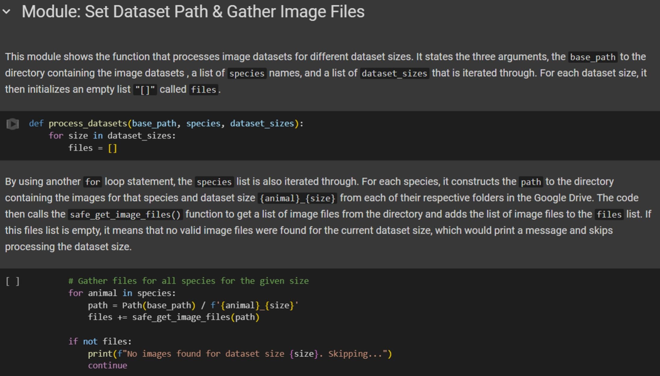
The Wild Winnipeg database consists of various animal classes that can be compiled into different dataset sizes. In particular, the dataset will include the fox, squirrel, and deer species involving 100, 500, 1000, and 5000 images for each class. These varying dataset sizes will be fine-tuned with Fastai and the pre-trained ResNet34 model. The model can be loaded by gathering local images for each species and its given size. More details about gathering the images and establishing directories for the script can be found in the Fastai Dataset Sizes Confusion Matrix Jupyter Notebook (figure 3.1).
Fine-tune the Model for Image Classification
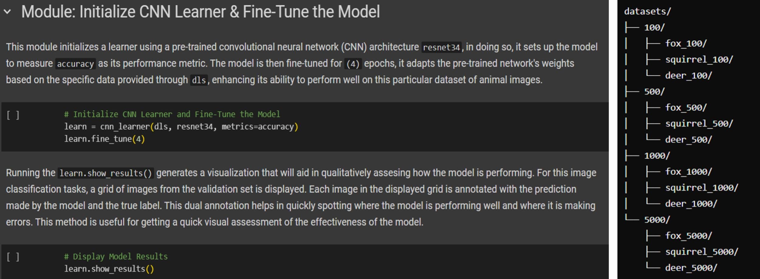
The fine-tuning script includes various features that demonstrate Fastai’s user-friendliness, streamlining the task of model training to a simplified deep learning process without compromising the use of advanced techniques. The metric of the model is focused on accuracy and set to as few as 4 epochs, adapting the network’s weights based on the specific datasets of animal images. The local dataset’s directory is structured as a single folder where each dataset size are in subfolders and can be located along with its labelled animal classes (figure 3.2). These images are processed through a single CNN learner which encapsulate complex operations into single, easy-to-use functions. In this way, users do not need to write extra lines of code for tasks like data augmentation, batching, or setting up the learning process. This abstraction allows for a quick setup that trains models without needing deep expertise in neural networks or optimization techniques. More details about the fine-tuning process itself can be found in the Fastai Dataset Sizes Confusion Matrix Jupyter Notebook, such as details about pre-processing, image data loaders, and file handling.
Confusion Matrices for each Dataset Size
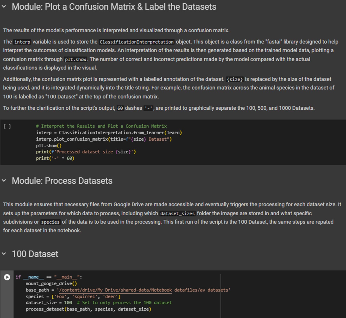
To display the model’s classification results and overall performance, a confusion matrix is plotted for each dataset size. A confusion matrix showcases the number of images a model predicts for a certain class and is plotted against its actual class, creating a grid of cells based on the model’s computational accuracy of classification. This approach focuses on using a ground truth as a foundational comparison to the model’s predictions, including True Positives (TP), True Negatives (TN), False Positives (FP), and False Negatives (FN). Therefore, matrices excel at providing insights into specific classification accuracies and errors. Under Fastai’s features and a pre-trained ResNet34 architecture, the objective is to create a matrix for each dataset size of 100, 500, 1000, and 5000 images. More details about how these visuals can be plotted to interpret model results are in the Fastai Dataset Sizes Confusion Matrix Jupyter Notebook (figure 3.3).
Model training also includes data metrics that represent the model’s performance in the task of image classification. These metrics are associated with terms such as accuracy, training and validation notes, as well as epochs. The definition of these metrics can be further understood in the glossary. Fastai’s visualization tools display the model’s training progress by showing validation losses and curves, as well as learning rate schedules for every epoch. At a small dataset size of 100 images, the model was already able to predict the fox, squirrel, and deer classes with a high level of accuracy. However, at a small dataset size, the accuracy starts quite low for the first epochs; it is not until the fourth and final epoch that the model reaches 94.8% in accuracy. As the model processes larger dataset sizes of 500, 1000, and 5000 images, the accuracy consistently stays at a high value for each epoch (figure 3.4).
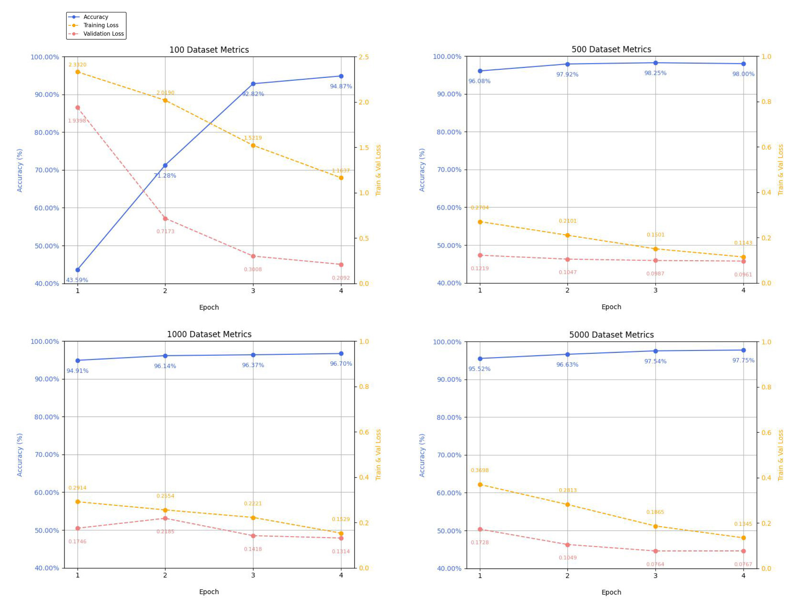
The average accuracy of the first epoch of these larger datasets is 89.4%. This, in comparison to the 41.5% accuracy of the 100 images’ first epoch, shows that the classification accuracy of Fastai and ResNet34 is more instantaneously and consistently accurate when it is dealing with larger dataset sizes. The overall accuracies of the larger datasets after 4 epochs are 98.2% for 500 images, 96.7% for 1000 images, and 97.8% for 5000 images. This significant decrease in accuracy of 98.2% to 96.7% from the 500 dataset to the 1000 dataset can be due to several factors. One reason to consider is the increase in dataset size. Even though all the images are of good quality and properly labelled, this increase in size may introduce more image variability in the dataset’s collection, which can affect model performance. Another reason to consider is that a larger dataset size can consist of a higher imbalance between specific classes, meaning there can be a varying distribution of images across different classes that constitute an imbalanced weighting of species, such as oversampling or under-sampling.[11] These results can be further visualized through the confusion matrices of each set. For instance, the 100 Dataset matrix shows that the model performs very well on deer and squirrel species with high true positives and relatively low false negatives (figure 3.5). The fox class may achieve good precision, but it still has the lowest performance due to its low number of true positives. These observations indicate that the model’s recognition of foxes could improve by augmenting the dataset of fox images.
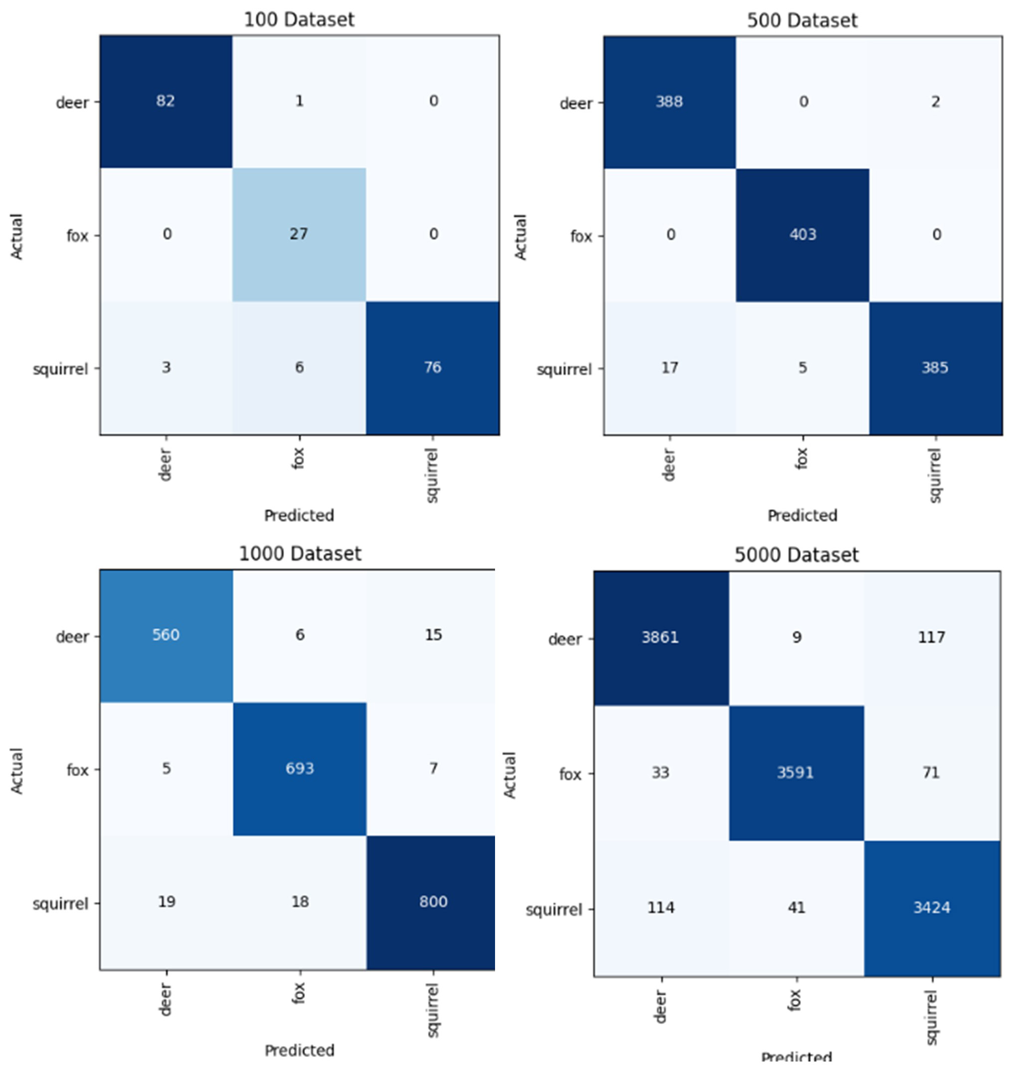
Figure 3.5: Confusion matrices for each dataset size of 100, 500, 1000, and 5000 images. These images were generated by the script in the Fastai Dataset Sizes Confusion Matrix Jupyter Notebook created by Zhenggang Li & A.V. Ronquillo.
Notes
- Abdallah Abbas, Khairil Imran, and Choo-Yee Ting, “User Experience Design Using Machine Learning: A Systematic Review,” IEEE Access 10 (January 2022): 1-1, https://doi.org/10.1109/ACCESS.2022.3173289. ↵
- Ibid. ↵
- Pascal Schröder, “Using Fastai for Image Classification,” Towards Data Science, June 14, 2019, https://towardsdatascience.com/using-fastai-for-image-classification-54d2b39511ce. ↵
- Jeremy Howard and Sylvain Gugger, “Fastai: A Layered API for Deep Learning,” Fastai Blog, August 13, 2021, https://www.fast.ai/posts/2020-02-13-fastai-A-Layered-API-for-Deep-Learning.html. ↵
- Fastai, “Fastai Documentation,” accessed July 13, 2024, https://docs.fast.ai/. ↵
- Howard and Gugger, "Fastai: A Layered API for Deep Learning." ↵
- Fastai, *fastai*, GitHub repository, last modified July 14, 2024, accessed June 28, 2024, https://github.com/fastai/fastai. ↵
- Ibid. ↵
- Ibid. ↵
- Kaiming He, Xiangyu Zhang, Shaoqing Ren, and Jian Sun, "Deep Residual Learning for Image Recognition," *arXiv*, December 10, 2015, https://arxiv.org/abs/1512.03385. ↵
- Sara Beery et al., "Synthetic Examples Improve Generalization for Rare Classes," *arXiv:1904.05916v2 [cs.CV]*, May 14, 2019, https://arxiv.org/abs/1904.05916. ↵
A branch of AI that enables computers to learn from data by analyzing patterns and trends in large datasets, using algorithms to make predictions, recognize objects, and generate new ideas based on learned information.
An open-source Python library built on PyTorch that focuses on making deep learning more approachable through user accessibility and abstractions. It provides easy-to-use APIs for training models and includes built-in functions for loading popular CNN architectures.
The underlying framework that Fastai is built upon, providing the foundational components for deep learning while Fastai adds additional user-friendly features and abstractions.
A type of neural network architecture particularly effective for image processing tasks. CNNs use convolutional layers to detect features in images and are commonly used in models like ResNet34 and as part of the Stable Diffusion architecture.
A 34-layer residual neural network architecture that is commonly used as a pre-trained backbone for image classification tasks, particularly effective when fine-tuned on specific datasets.
A large dataset commonly used for pre-training models like ResNet34, containing millions of labeled images across thousands of categories.
A parameter that determines the number of complete passes through the entire training dataset the model will undergo during training. The number of epochs significantly influences the number of computational resources and time required for training. More epochs can lead to better model performance but may also increase the risk of overfitting.
The process of teaching a machine learning algorithm to make accurate predictions by feeding it labeled data examples, allowing the model to learn patterns and relationships that enable it to classify or predict outcomes on new, unseen data. This involves adjusting the model's internal parameters through iterative exposure to training data until the model achieves satisfactory performance.
Parameters within the model that are adjusted during the fine-tuning process. Fine-tuning involves modifying pre-existing weights. In contrast, training a custom model requires initializing and adjusting new weights.
A built-in feature of YOLOv8 model training that involves manipulating aspects of the training images to increase model accuracy and generalizability. This is done by modifying image saturation, hue, orientation, or noise levels, amongst other characteristics.
A parameter determining the number of images used simultaneously in each epoch during model training. It can be adjusted by the user and impacts the speed of the training process. The minimum batch size for fine-tuning the YOLOv8 model is 8.
A visualization tool that showcases the number of images a model predicts for a certain class plotted against its actual class, creating a grid of cells based on the model’s computational accuracy of classification. It displays True Positives (TP), True Negatives (TN), False Positives (FP), and False Negatives (FN) to provide insights into specific classification accuracies and errors.
Instances where the model correctly identifies a positive case that exists in the ground truth data.
Instances where the model correctly identifies the absence of a positive case in the ground truth data.
Instances where the model incorrectly predicts a positive case when none exists in the ground truth data.
Instances where the model fails to identify a positive case that actually exists in the ground truth data.
The simplest image analysis technique offered by YOLOv8, image classification involves identifying what class the objects within a given image belong to and provides the class name and confidence score. This technique does not identify the location of the predicted objects within a given image.
A metric that measures how well a model performs on data it hasn’t seen during training, used to monitor model performance and detect overfitting during the training process.
A technique used to address imbalanced datasets by increasing the number of examples in minority classes, often through methods like synthetic image generation, to create more balanced representation across all classes during model training.
A technique used to address imbalanced datasets by reducing the number of examples in majority classes to create more balanced representation, though this approach risks losing potentially valuable training data.
The percentage of true positives within all positive predictions made by the model. This metric indicates model accuracy in predicting specific classes.
