5.1 Types of Maps

Geologists and geophysicists are also interested in the Earth’s surface and the distribution of materials. They use maps as tools to visualize data in an area, including elevation, rock type, groundwater levels, hazards, and pollution, among other data.

There are three basic map types: planimetric, topographic, and thematic.

1. Planimetric maps are the most familiar to people; they are the usual city or provincial maps you see. They show a two-dimensional view of the Earth, including features such as lakes, rivers, and cultural features, such as roads, cities, and political boundaries.
2. Topographic maps are one of the most useful maps to geologists. These generally include planimetric map features, plus information about the three-dimensional appearance of the Earth’s surface using contour lines. In Canada, many topographic maps use maps produced by the Government of Canada, under the National Topographic System (NTS).
3. Thematic maps are another useful map that shows a specific topic, such as population density distribution or ocean floor depth. The thematic map we will use is a geologic map, which shows the distribution of rock units in an area. Geologists also commonly use other thematic maps, such as those that show locations of aquifers or risk assessments for natural hazards.

Regardless of the type of map, they all require certain features. These include a scale, a directional indicator, and a way to designate location.

5.2 Map Scales

Maps are scaled-down versions of the Earth’s features so we can view them in a workable form. “Scale” refers to the amount of reduction the map represents. All maps include at least one type of map scale to compare the distance between two points on the map with the distance between the same two points in real life. Scale may be expressed as a fractional, graphic, or verbal scale.

Fractional (or Ratio) Scale

The fractional scale is the ratio of “map” distance to “real-world” distance. A typical fractional scale is 1:50,000, which means 1 unit of measure on the map is equal to 50,000 of the same units of measure on the ground. In other words, 1 cm on the map is equal to 50,000 cm on the Earth’s surface, or 1 metre on the map is equal to 50,000 metres on the Earth’s surface, etc. Notice that “1:50,000” itself does not have units; it is a ratio. Fractional scales can be applied equally to metric or imperial measurements, as long as both sides of the ratio have the same units (e.g. both in metres, or both in centimetres, or both in feet, or both in miles, etc.). A map with a scale of, for example, 1:20,000 will show a smaller area with greater detail, and is called a large-scale map. On the other hand, a map with a scale of 1:1,000,000 will represent a larger area with less detail, called a small-scale map.

5.1 Examples on Fractional Scale Conversions

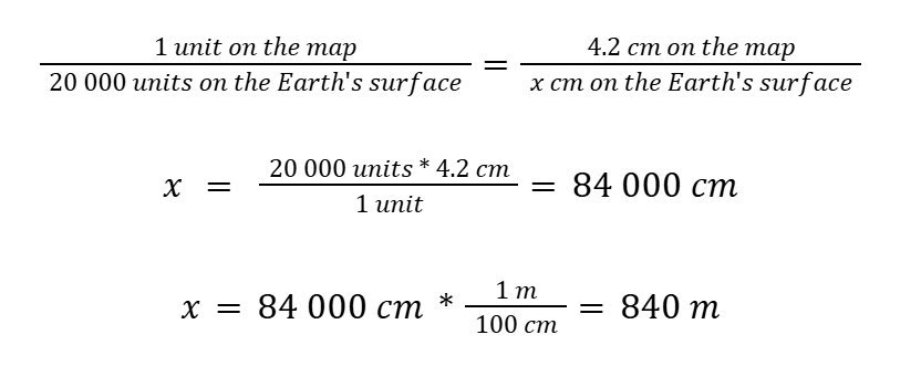
• If the distance between points on a 1:20,000 map is 4.2 cm, what is the actual distance (x) on the Earth’s surface?

• You are given a bar that represents a distance of 1000 metres, which measures to 4 cm. What is the fractional scale of the map?

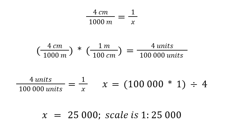
Saying 50,000 m on Earth’s surface is unusual; you would more likely measure this as 50 km. Measuring a metre on a page-sized map would also be unusual; you would measure map distances in centimetres. To use fractional scales, you need to have both sides in the same units before calculation.  Note how in the examples above, both the numerator and denominator have the same units, unless converting.

Graphic scale

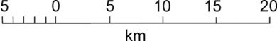
A graphic scale consists of a line or bar corresponding to a kilometre or some multiple or fraction of a kilometre (Figure 5.3). This scale is easy to visualize, commonly used, and will keep its true proportions if the map is enlarged or reduced (such as with a photocopier). The graphic scale provides a convenient way of measuring distances on a map. To find the distance between two points on a map, use a ruler to measure the distance and then compare it to the length on the graphic scale. If you need to measure a curved path, lay a string along the path, then measure the length of the string, and then compare the measurement to the graphic scale.

Verbal scale

Early Canadian maps were scaled as “so many inches per mile”. For example, a map with the verbal scale “one inch per quarter mile” would mean that a measurement of one inch between two points on the map represents a real-world distance of 0.25 mile. This type of verbal scale is rarely used on modern maps but exists on older maps.

5.3 Direction

Understanding geographic orientation is an important skill in using maps. You may want to know the direction a rock unit is oriented, or the direction a river used to flow. There are three forms that you should be aware of: the cardinal directions, the azimuth system, and the quadrant bearings.

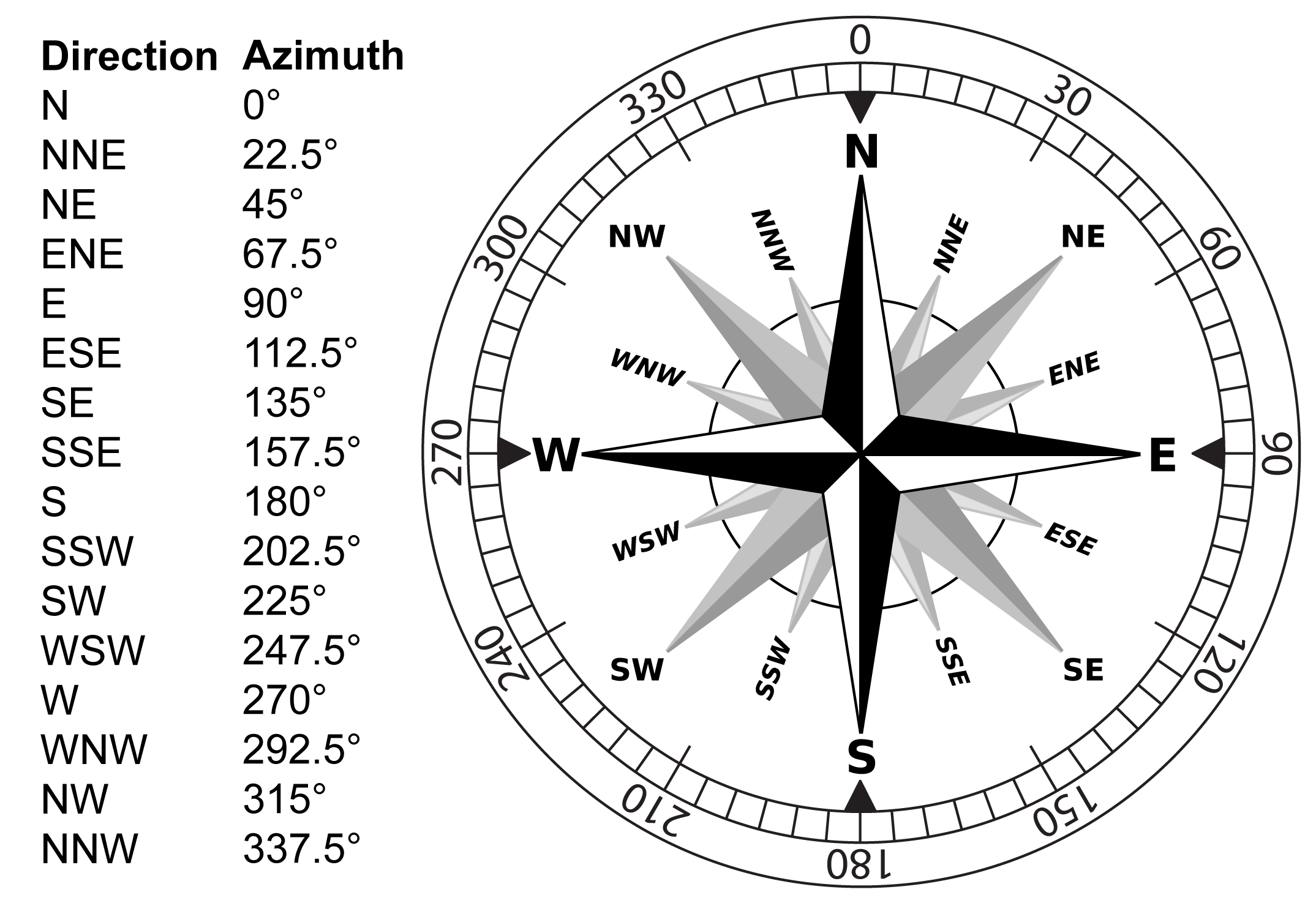
The cardinal directions refer to names we already know: North, South, East, and West. These may be subdivided into intercardinal directions, such as NNE, NE, ENE (Figure 5.4). Maps will typically be oriented so the top of the map points towards geographic north, or true north (we will return to this!). However, the top of the map is not always north; therefore, north is usually indicated on maps with a north arrow, which can also be helpful to measure angles accurately. Some maps may use an ornate compass, although it is preferred to use a simple arrow labelled with “N” at the end of it.

Bearing

The cardinal system is not very exact, which is why we use two bearing systems. Indicating direction from one point to another is done with a degree measurement called a bearing. A compass measures the angle between north and the direction that the compass is pointed in degrees. We may express those measurements as either an azimuth or a quadrant bearing (Figure 5.4).

In the azimuth system, directions are given as the number of degrees clockwise from0º to 360º. North is 0º, east is 090º, south is 180º, and west is 270º. Azimuth measurements are always expressed as a three-digit number with the degrees symbol (for degrees <90, this would be presented, for example, as 055º, instead of 55º).

Quadrant bearing measurements subdivide direction into four quadrants (northeast, southeast, southwest, northwest), each covering 90º. The quadrant measurement is indicated as the number of degrees east or west from north, e.g., N50ºE, or south, e.g., S27ºW.

Magnetic Declination

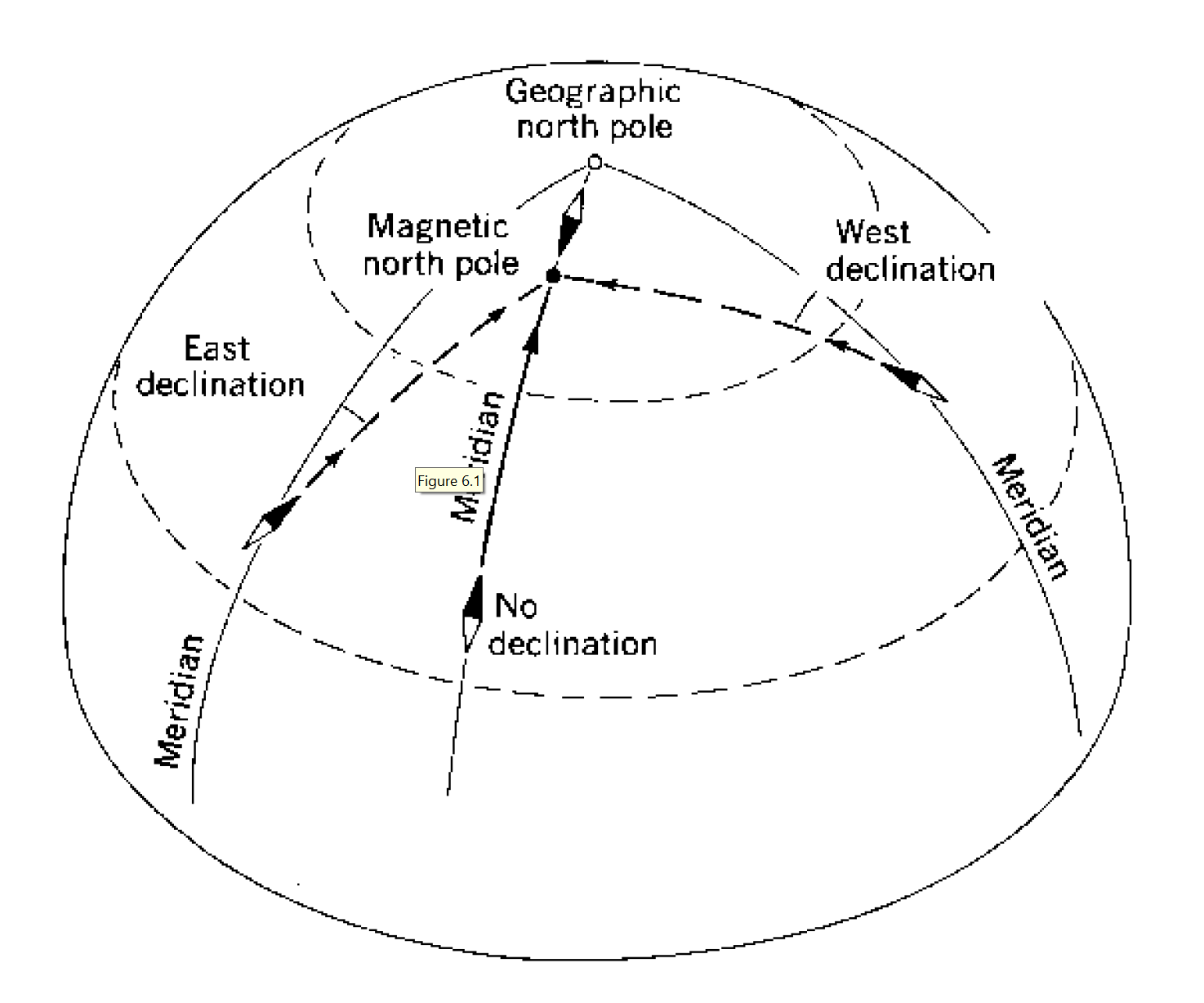
Direction on a map is measured to true (geographic) north. However, a compass points to the magnetic north pole. Because magnetic north is located at a different position on Earth than true north, you must account for this difference by using the magnetic declination, which is the angle between true north and magnetic north. The declination can vary from 0° to 180°, depending on the geographic location where the measurement is taken to the two poles (Figure 5.5). The poles will also change, or wander, constantly. Over time, slight corrections are made to account for this wander. Government-issued maps, such as NTS maps, include information on how to account for changes in magnetic pole position that have occurred since the map was published.

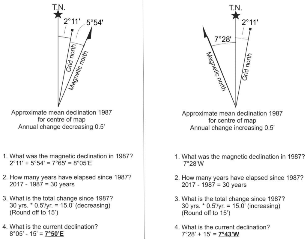
5.2 Examples on Magnetic Declination Calculation

In Figure 5.6, calculate the magnetic declination for the year 2017 from these two different declination diagrams.

Exercise 5.2 – Map Directions

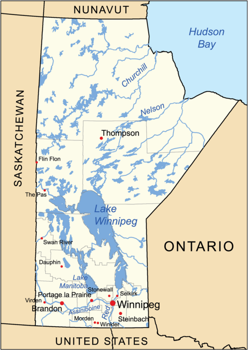
Test your knowledge using Figure 5.7:

a. Without using a protractor, what is the cardinal direction between the following cities?

i. Winnipeg to Brandon

---

ii. Thompson to The Pas

---

iii. Portage la Prairie to Steinbach?

---

iv. Virden to Stonewall?

---

v. Flin Flon to Swan River?

---

vi. Dauphin to Swan River?

---

 

b. Now use a protractor to find the azimuth direction for the following cities.

i. Winnipeg to Brandon?

---

ii. Thompson to The Pas?

---

iii. Portage la Prairie to Steinbach?

---

iv. Virden to Stonewall?

---

v. Flin Flon to Swan River?

---

vi. Dauphin to Swan River?

---

5.4 Coordinate Systems

An essential skill that a geologist needs is the ability to locate places on maps. In this course, we use 3 coordinate systems to describe positions on a map. These are Latitude and Longitude, Universal Transverse Mercator (UTM), and Dominion Land Survey.

Latitude and Longitude

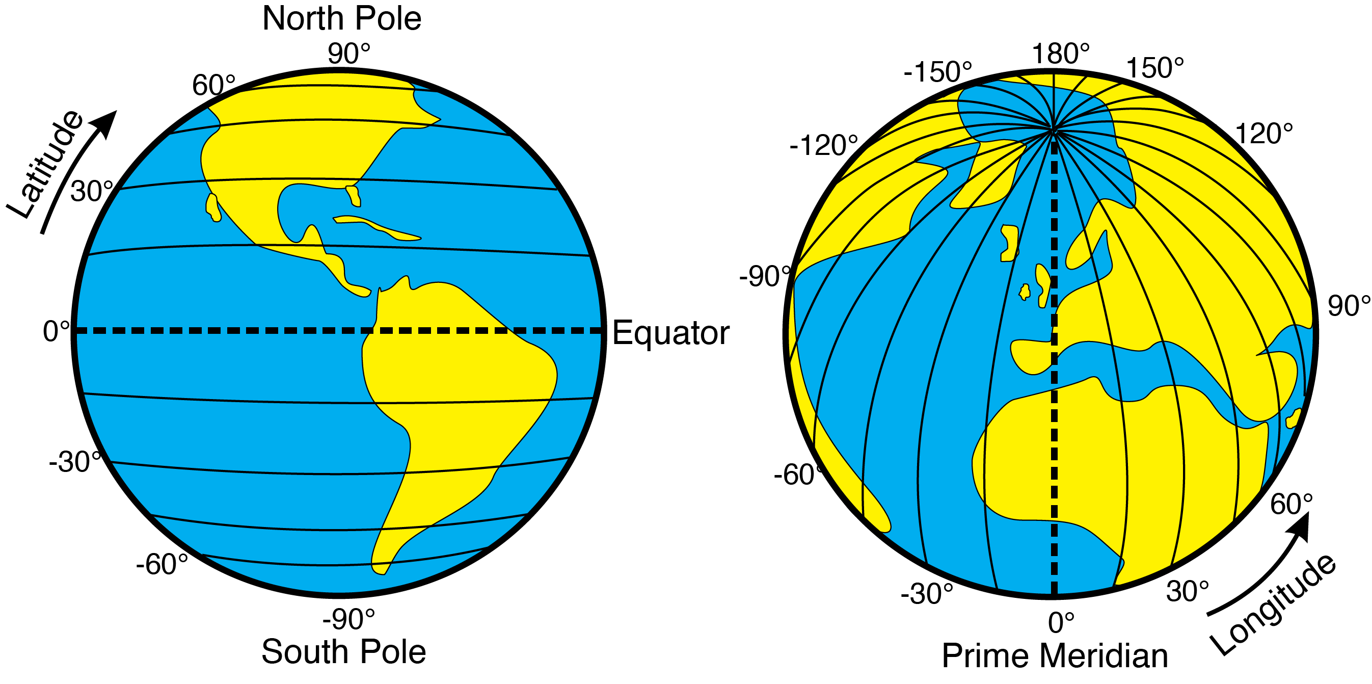
One of the most common methods used is latitude and longitude (Figure 5.8). To note the location of a point on Earth, two coordinates are needed: (1) latitude, which gives the north-south position, and (2) longitude, which gives the east-west position.

Latitude measures how far north or south a location is from the Earth’s equator. The equator lies at 0° latitude, which increases to 90° north (the north pole) or 90° south of the equator (the south pole). Latitudes between the equator and the North Pole are part of the northern hemisphere, and latitudes between the equator and the South Pole are the southern hemisphere. Lines of latitude (parallels) run horizontally and remain parallel to each other (Figure 5.8). For example, the 49th Parallel north, at 49°N, forms part of the border between Canada and the United States. One degree of latitude covers ~111km; therefore, we use minute and second subdivisions to precisely describe locations.

Lines of longitude (meridians) are curved, imaginary lines that circle the globe, passing through the north and south poles (Figure 5.8). The 0° longitude line, or the Prime Meridian, passes through the town of Greenwich, England, and extends to 180° in both directions east and west of the Prime Meridian to the 180° longitude line that passes through the Pacific Ocean. Locations west of the Prime Meridian to 180° are in the western hemisphere; those east of the Prime Meridian to 180° are in the eastern hemisphere. The International Date Line corresponds to 180° longitude (with some irregular jogs added for political convenience). When measured on the Earth’s surface, one degree of longitude varies from about 111 km at the equator to 0 km at the poles, where the meridians intersect. As with latitude, the subdivisions of minutes and seconds are used in most location descriptions of longitude.

Here is an example of our location expressed by its latitude and longitude:

49°48’42”N (latitude) 97°08’09”W (longitude)

Combining latitude and longitude provides a unique coordinate to every point on Earth’s surface. For example, Mt. Fuji in Japan is located at about 35°N 138°E. A more precise location for Mt. Fuji is 35°21′38″N 138°43′39″E. This coordinate system is in degrees (°), minutes (‘), and seconds (“), also known as DMS. Degrees range from 0 to 90, while minutes and seconds range from 0 to 60. Another way to display these spherical coordinates is using decimal degrees (DD). Those same coordinates for Mt. Fuji using decimal degrees are 35.36056°N 138.72750°E. While DMS is the classic way of representing coordinates, decimal degrees are easier when creating maps and plotting data with software.

Universal Transverse Mercator (UTM)

The Universal Transverse Mercator System, or UTM system, is widely used. In recent years, it has been widely used in hand-held GPS (Global Positioning System) receivers for commercial and recreational uses, and the widespread use of GIS (Geographic Information System) software.

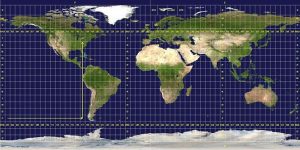
The UTM system employs uniform grids, in which the lines are evenly spaced, like the fabric of a screen. In the UTM system, the world is divided into 60 zones, each 6° wide (Figure 5.9). To see why the UTM system divides the world into all these zones, remember that the Earth is an oblate spheroid, with flattened poles and a bulging equator. Imagine trying to align a piece of screening on a basketball: it is not possible to do so without wrinkles and distortion. The narrow slices of the individual zones are designed to reduce distortions caused by overlaying a two-directional grid onto a spheroid. On maps where the Earth’s surface is projected to look like a rectangle, the zones also look like rectangles. In actuality, the shape of the zones more closely resembles the shape of the outer surface of a segment of an orange. Being curved in this way, the width of each zone varies considerably: at the equator, a zone is 666 km wide; at 80°N latitude, the same zone is only 80 km wide.

The UTM grid is measured in square metres. As with all two-directional grids, a point is located by both an X coordinate and a Y coordinate. The Y coordinate, or Northing, increases northwards from 0 at the equator to 10,000,000 metres at the North Pole. The X coordinate, or Easting, is arbitrarily assigned as 500,000 metres at the centre of each zone and extends from 0 metres in the west to no more than 999,999 metres to the east of that central meridian. This numbering scheme was developed to avoid the use of negative numbers.

Here is a typical representation of a UTM coordinate for a point:

635290m E           5519370m N  Zone 14

Eastings are traditionally listed first. Co-ordinates are noted with the unit “m”, the standard abbreviation for metres. Zone numbers are included, an essential part of the coordinate.

Dominion Land Survey (AKA Public Land Survey or Township-Range System)

The Dominion Land Survey (DLS) is used to describe land locations across the Prairie provinces of Canada and parts of the US Midwest and West. It was originally developed in the late 1800s to organize land for homesteading and has since been widely used in agriculture, the petroleum industry, and defining municipal boundaries.

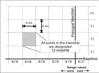
The DLS system divides land into square units called townships, each measuring 6 miles by 6 miles (36 square miles). Townships are numbered by their position relative to two types of reference lines: meridians (north-south lines) and baselines (east-west lines) (Figure 5.10).

In Canada, the Principal (or 1st) Meridian was placed just west of Winnipeg. Additional meridians (2nd, 3rd, 4th, etc.) were established about 4° of longitude apart as you move west. The range is the number of six-mile strips east or west of a meridian, noted as “R” (e.g., R2W3 means two ranges west of the 3rd meridian).

Baselines mark the position northward from a reference latitude; notably, the 1st Baseline, which follows the 49th parallel, Canada’s southern border with the US. Townships north of this baseline are numbered as “T”, “Tp”, or “Twp” (e.g., T3N means 3 six-mile units north of the 49th parallel).

Since the Earth is curved, the width of a township along the northern boundary is slightly smaller than at the southern boundary and going northwards worsens the issue. Therefore, east-west correction lines were added periodically to adjust the grid and keep township areas roughly equal, resulting in slight jogs in roads or land boundaries.

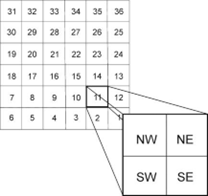
Each township is further divided into 36 sections (1 square mile or 640 acres each), which can then be subdivided further into quarter sections (160 acres), labelled NE, NW, SE, or SW (Figure 5.11).

A typical representation of a DLS coordinate will follow this order:

Quarter (NE, NW, SE, SW) – section (1-36)- township (#) -range (#) – (E/W of a given meridian)

Here is an example of a DLS coordinate for a point:

NE-08-10-3EPM  or    NE1/4, sect. 8, T10, R3 EPM

For this example, it means that the land is located in the NE quarter of section 8, township 10, range 3, east of the Prime Meridian.

Here is another example:

SE-20-12-9W4   or     SE1/4, sect. 20, T12, R9 W4

For this example, it is in the SE quarter of section 20, township 12, range 9, west of the 4th Meridian.

Exercise 5.3 – Converting Geographic Coordinates

Figure 5.12 shows you how to convert a single coordinate back and forth between DMS and DD.

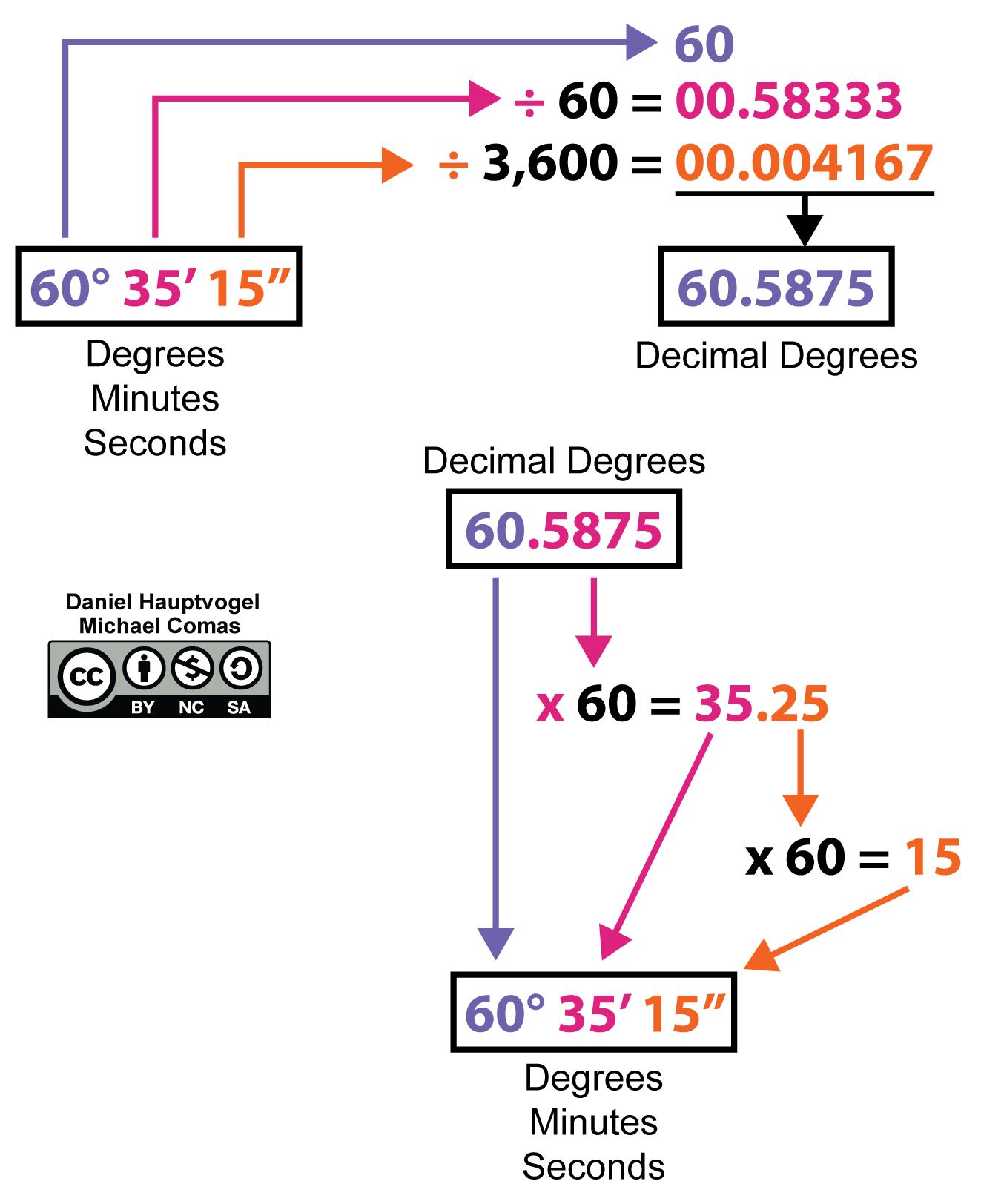
1. Table 5.1 contains geographic coordinates for some cities, as shown in Figure 5.13. One of the coordinate systems is given for each city. Using Figure 5.12, convert coordinates to either DMS or DD. Winnipeg, MB, has been done for you.
   

   Table 5.1 – Canadian cities and their geographic coordinates

   	Degrees Minutes Seconds (DMS)	Decimal Degrees (DD)
   Winnipeg, Manitoba	49°53’04” N 97°08’49” W	49.8844° N 97.1470° W
   Ottawa, Ontario	45°24’40” N 75°41’53” W	45.4112° N 75.6981° W
   Iqaluit, Nunavut	63°44’49” N 68°31’2″ W	63.747° N 68.5173° W
   St John’s, Newfoundland and Labrador	45°16’15” N 66°3’22” W	45.2708° N 66.0562° W
   Edmonton, Alberta	53°33′ N 113°28’7″ W	53.5501° N 113.4687° W
   Whitehorse, Yukon	60°43’16” N 135°03’24.5″ W	60.7212° N 135.0568° W
   Toronto, Ontario	43°39’11.5″ N 79°22’59.5″ W	43.6532° N, 79.3832° W

2. Which coordinate system do you think is better and why?
   

   ---

   ---

5.5 Contour Lines and Topographic Maps

Topographic maps show the shape and elevation of the Earth’s surface, known as topography. Topographic maps use contour lines to show elevation changes. Contour lines connect points with the same elevation on Earth’s surface, with reference to the vertical distance above (or below) sea level.

There are some rules when reading or drawing contour maps.

Contour lines represent areas of equal elevation on a map; every point along a given contour line is at the same height above sea level. These lines will always form closed loops, even if part of the loop continues off the edge of the map. Contour lines do not cross, split or merge, except in rare cases like vertical cliffs.

The shape and spacing of contour lines show the shape of the land: closely spaced lines indicate steep slopes, while widely spaced lines indicate gentle ones. Evenly spaced lines show a constant slope.

Areas enclosed by contour lines are at a higher elevation than the contour’s value, while elevations between lines are estimated by assuming a steady slope. For example, a point halfway between 20m and 30m contours will be about 25m.

Depressions (sunken areas) are shown with contour lines marked with hachures  (short lines that point down the slope); the first hachured line will share the same elevation as the previous regular contour. When two adjacent contour lines have the same elevation, it marks a slope reversal (such as a ridge top or a valley bottom).

Every fourth or fifth contour is darker and labelled, called index contours, which are used to estimate the values of unlabeled lines. This is to avoid clutter within the map. Precise elevation points (spot elevations) are marked with an “X” or “+” and a number, and extremely accurate elevations (benchmarks) are shown with an “XBM”. When contour lines cross a river or valley, the line forms a “V” shape. The open side of the V is towards the lower elevation/downstream, and the point of the V points towards the higher elevation/upstream. This is called the Rule of V’s.

Most of us now use our cell phones with built-in GPS, maps and apps to help us decide where to go. Even with these, you hear stories of people blindly following these and ending up on roads that dead-end or are closed due to weather. Or you may go someplace without a cell signal to be able to use your map app. So, knowing how to read a topographic map is a useful skill for these and other situations.

5.6 Topographic Profiles

A topographic profile is a side view or cross-section of the land surface along a specific line on a topographic map. It shows how elevation changes across the landscape and helps visualize terrain shape, slope, and relief.

The horizontal scale of a profile matches the scale of the map. The vertical scale can be the same for a true-to-scale profile, but it’s often exaggerated to make elevation changes more visible. This is called vertical exaggeration (V.E.), and it’s calculated as:

V.E. = horizontal scale ÷ vertical scale

For example, if the map scale is 1:50,000 and the vertical scale is 1:5,000, the V.E. is 10×. Be sure to convert both scales into fractions (e.g., 1:50,000 = 1/50,000) before calculating.

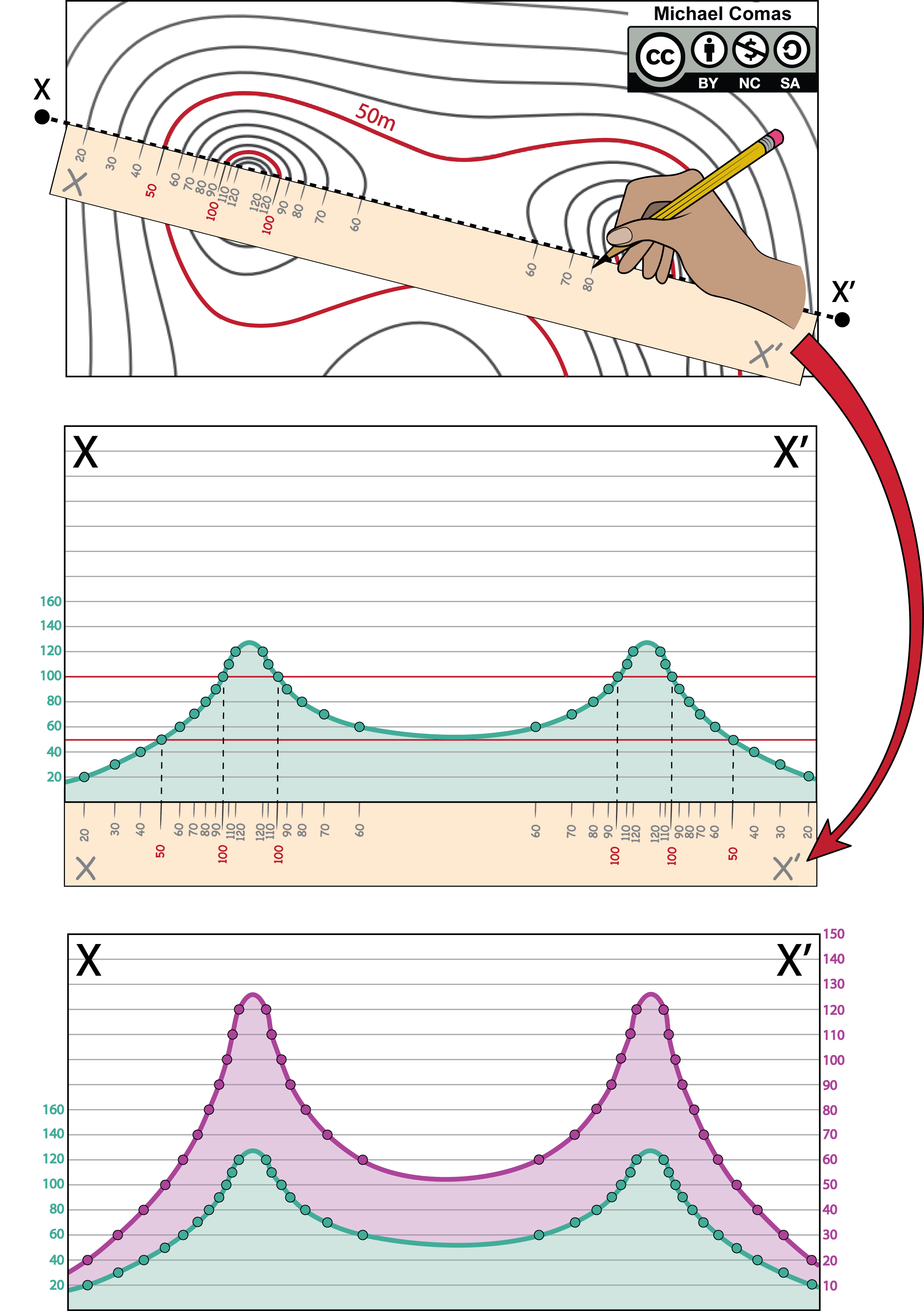
Steps to Construct a Topographic Profile

To get a good sense of the landscape, geologists construct topographic profiles (Figure 5.15). To do this, use these five steps:

1. Draw a Line on the Map
   Choose or follow the given line (e.g., A–B or X–Y) across the area of interest. (Figure 5.15)

2. Mark Elevations on a Scrap Strip
   Place a piece of paper along the line, mark where contour lines cross it, and record the elevation at each point. Also note features like streams or roads.

3. Set Up the Profile Axes
   On graph paper or the provided template, draw the vertical axis using an appropriate vertical scale (e.g., 1 cm = 100 m), with enough range to include the highest and lowest elevations. The horizontal axis should match the map scale and length of the line.

4. Plot and Connect Points
   Transfer the elevation points from your scrap strip to the profile. Use smooth, curved lines (not sharp or straight ones) to connect the points. Mark any features, like rivers, that cross the profile.

5. Calculate and Label Vertical Exaggeration
   Using the scale values, calculate the V.E. and clearly label it below the profile.

Note: Vertical exaggeration enhances the visibility of topographic changes but also alters the natural appearance of the landscape, so interpret with care.

Exercise 5.4 – Maps and Topography

Your instructor will provide you with the map required for this question.

Question 1. Use the National Topographic Systems Map Baldur to answer the following questions.

        a. What is the (fractional) scale of the map? ____________________________________

        b. How much latitude and longitude (in minutes) does the map cover? ___________________

        c. What is the contour interval? ____________________________________________________________

        d. What is the NTS map sheet number? ____________________________________________________

        e. Which UTM zone covers this map sheet? ________________________________________________

What is the distance represented between each of the thin blue grid lines on the map?                _____________________________________________________________________________________________

        f. What type of data was used to produce this map? ____________________________________________

        g. If you were setting the magnetic declination on your compass for work in this area in 2017, what declination would you use? _______________________________________________________

        h. For points marked A and B on the map, give their coordinates:

     I. latitude & longitude (degrees, minutes, seconds),

        A: ________________________________________  B: _____________________________________________

     ii. UTM coordinates,

        A: ________________________________________  B: _____________________________________________

     iii. township & range coordinates,

        A: ________________________________________  B: _____________________________________________

        i. What is the distance (direct, straight line) between points A and B? _____________________

        j. What is the driving distance between points C and D? (Use roads, not tracks or trails.) ________________________________________________________

        k. In which Rural Municipality does the town of Baldur occur? _____________________________

        l. What do the dashed lines around the lakes on this map sheet indicate? ___________________________________

        m. Which way does Oak Creek flow near Sveinsson Lake? _________________________________

 

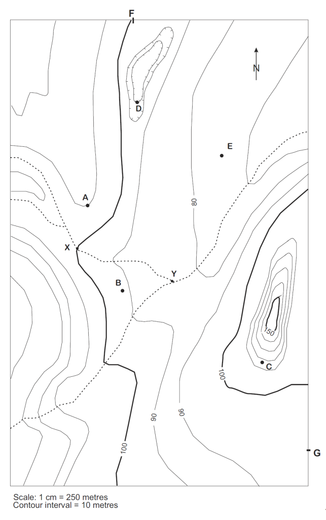
Question 2. Use the topographic map shown in Figure 5.16 to answer the following questions. The solid lines are contour lines, and the dashed lines are streams.

        a. Determine the elevation for the unnumbered contour lines and mark them along those lines, neatly, in the same fashion as the other contour lines. Note that numbers on contour lines are oriented upright towards higher elevations.

        b. Put a coloured L on the lowest point in the map area. What is its approximate elevation?

            Why isn’t the elevation of L = 70m? to 60 m?

            Put a coloured H on the highest point in the map area. What is its approximate elevation?

        c. What is the elevation at the following points:

    A: __________________________________________

    B: __________________________________________

    C: __________________________________________

    D: __________________________________________

    E: __________________________________________

        d. How do you calculate the relief of an area from a map? What is the approximate relief of this map’s area? (Use the elevations calculated in Q1b)

        e. Name 3 indicators that allow you to determine the direction of stream flow.

1. _____________________________________________________________________________
2. _____________________________________________________________________________
3. _____________________________________________________________________________

           Draw coloured arrows along each branch of the stream to show the direction of stream flow. (The arrows should point toward the downstream direction.)

        f. What is the gradient of the stream branch between points X and Y? Show your calculations.

        Expressed verbally (complete the expression: 10 metres per ______________________________

        Expressed as a percent: ____________________________________

        g. At the bottom of the map, draw a graphical scale that is equivalent to the verbal scale shown. Make your scale represent 1 km distance. What would be the fractional scale for this map?

_________________________________

        h. Draw a straight line to connect points F and G on the map. On a piece of graph paper, draw a topographic profile along the line F-G using a vertical scale of 1 cm = 20 metres.

        i. For the topographic profile you have drawn, what is its vertical exaggeration? Show your calculations. _______________________________

        j. Assume that you are making a traverse from Point A, then to Point B, then to Point C, then to Point D, then to Point E. Go directly from one point to another. Fill in Table 5.2 to give the direction and distance that you would travel on each leg of this journey.

Table 5.2 – Direction and distance between selected points. 

	Direction (Azimuth measurement)	Direction (Quadrant measurement)	Distance (km) (report to 3 decimal places)
A-B
B-C
C-D
D-E

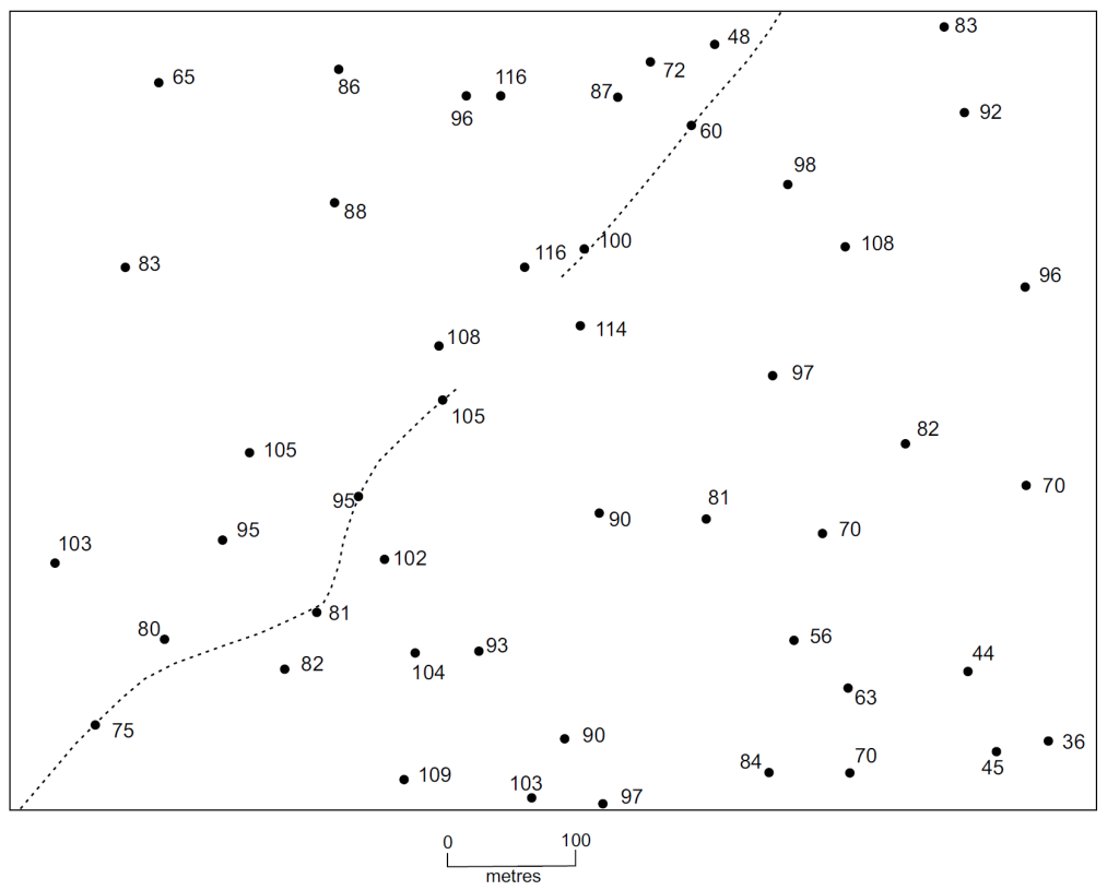
Question 3. Use Figure 5.17 for this question. The numbered points on this map represent elevations (in feet above sea level). The dashed lines are streams.

1. Draw the contour lines for this map using a contour interval of 20 metres. (Convention: Contour in even-numbered intervals, such as 0, 20, 40, 60… instead of 10, 30, 50…)
2. Draw arrows along the streams to indicate the direction of stream flow.
3. Note that a graphic scale is provided below this map. What is the fractional scale of this map? _____________________________________________

Additional Information

Exercise Contributions

Lab 5: How Do You Look at the Earth’s Surface? was modified by Jessica Kristof and Ricardo L. Silva from the original Chapter 1: Introduction to Science and Geology by Daniel Hauptvogel, Virginia Sisson, Michael Comas, and Somaria Sammy, and Chapter 2: Topographic Maps by Michael Comas, Daniel Hauptvogel, and Virginia Sisson in Hauptvogel et al., (2024) and from the original Lab 5: Maps & Topographic Maps in Ferreira and Young (2018). 

References

Ferreira, K. and Young, J. (2018). GEOL 1340 The Dynamic Earth Lab Manual. Winnipeg, MB: Department of Geological Sciences, University of Manitoba

Hauptvogel, D., Sisson, V., and Comas, M. (2024). Investigating the Earth: Exercises for Physical Geology. Houston, TX: UH Libraries