Lab 6: Why Do The Red and Assiniboine Rivers Look Like They Do?
Drainage Basins, Meanders, and Flooding
Learning Objectives
The goals of this chapter are to:
- Understand drainage basins and river patterns
- Interpret meandering rivers using maps and a stream table
- Construct and evaluate hydrographs
6.1 Drainage Basins
Rivers are an important part of the hydrologic cycle as they provide much of the water that is essential for our existence. They provide food, freshwater, and fertile land for growing crops. While water is vital to life, it can also be a destructive force when rivers flood. Rivers are responsible for creating much of the topography that we see around us through erosion and the transport of sediment.
The area that water flows to form a river is known as a drainage basin, or watershed. All of the precipitation (rain, snow, etc.) that falls within a drainage basin eventually flows into its stream, unless some water crosses into an adjacent drainage basin via groundwater flow. In an ideal scenario, when a single raindrop falls on the Earth’s surface, gravity drives it, along with other drops, downslope until it reaches a small stream (tributary). This stream meets a river, and this river will flow into more rivers until it reaches a basin, lake, or ocean. This means that where the drop falls will determine where it flows. In Canada, the Snow Dome in Jasper National Park drains water into the Pacific Ocean, the Arctic Ocean, and Hudson Bay.
Exercise 6.1 – Discovering Drainage Basins
One great tool for visualizing this process across the globe is River Runner Global. This website allows you to drop a single drop of rain anywhere on Earth, and River Runner will determine which path it will take to the ocean.
Your instructor will choose 6 of the 18 points provided on the map in Figure 6.1 for the drop start point. Drop it as close as possible to the number on the map. For each drop, River Runner will provide statistics and show you the path your drop would take. Do not choose all six points from one region.

Refer to Figure 6.1 to complete the following questions.
- Before placing any drops, do you think a drop will always end up in the ocean? Why or why not?
- In Table 6.1, record the location number, province, number of rivers (and lakes) the drop passes through, the total distance travelled (km), the river that the drop travelled the longest distance in, and the basin it ended up in.
Table 6.1 – River Runner data No. Province Number of Rivers Total Distance (km) Longest River Final Basin - Did you notice any rivers that appeared multiple times in your paths? Which ones? Why do you think that is?
- Place a drop on each of the blue points in Alberta. In which basins do the three drops end up? Why do you think this is, considering they are so close to one another?
- Critical Thinking: Why can some drops travel hundreds of kilometres through only one or two rivers, while others travel tens of kilometres through many rivers?
The movement of water in a stream is driven by gravity, so streams will only flow downhill. We have already learned that moving water is one of the mechanisms for weathering and erosion. Streams weather the materials around them and transport the sediment downstream, leaving behind channels, valleys, and other landscape features. However, many factors can affect how streams shape a landscape, including gradient, flow velocity, amount of water, sediment load, and channel shape and roughness.
The pattern of a stream system is determined by the geology of the underlying material. Is the stream moving over rock or soil? Are there faults, fractures, or other geologic structures?
Exercise 6.2 – Observing Stream Patterns
Instead of following a drop of water, observe satellite images of steam networks. Figure 6.2 contains Google Earth Images of four streams with different channel patterns, and Figure 6.3 shows the same streams in black and white. These patterns have specific names, but the goal is for you to recognize and describe these patterns on your own.
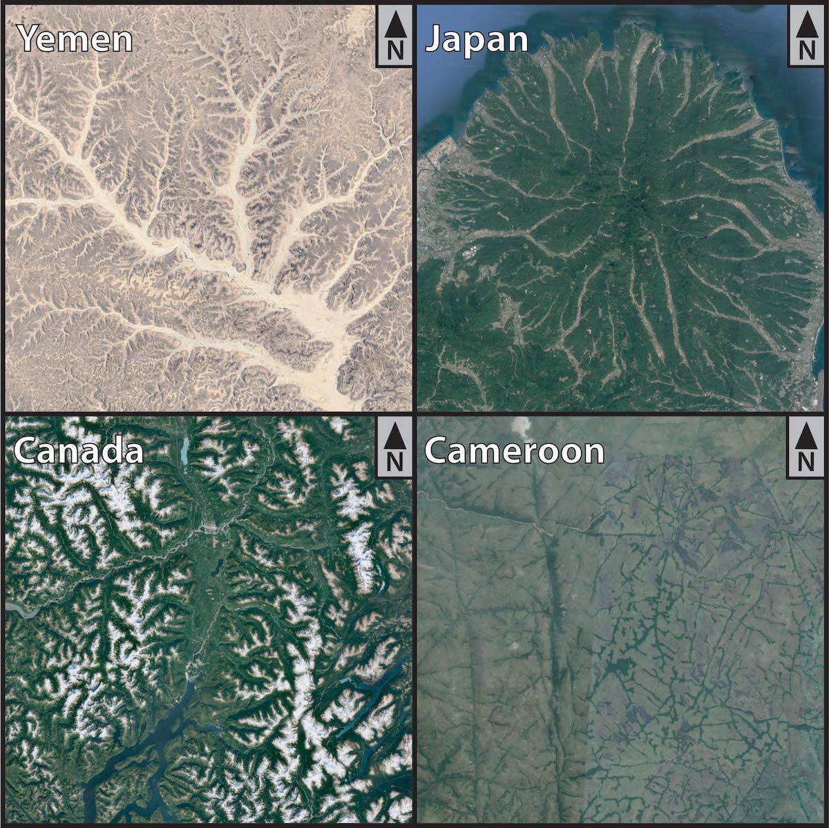
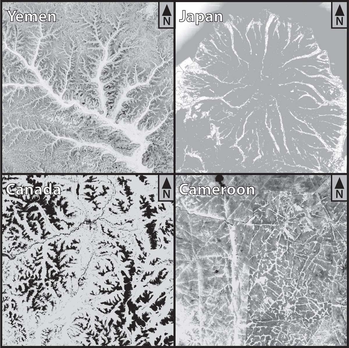
- Look at the patterns for each stream. Trace the patterns in Figure 6.3 and then describe the drainage patterns.
- Yemen:
- Japan:
- Canada:
- Cameroon:
- Yemen:
- What do you think is causing the patterns you observed in each stream?
- Yemen:
- Japan:
- Canada:
- Cameroon:
- Yemen:
- Critical Thinking: Do you think some stream types are more common than others? Why?
6.2 Alluvial Fans
An alluvial fan is a deposit of sediment that forms when a high-gradient (high slope) stream flows out of a narrow, high-elevation valley onto a flatter plain. As the stream loses energy on the flat land, it slows, spreads out, and drops sediment in the characteristic fan shape. Alluvial fans typically form where a flow of sediment or rocks emerges from a confined channel and is suddenly free to spread out in many directions.
Exercise 6.3 – Alluvial Fans
Your instructor will provide you with an aerial photo and stereopair glasses.
How to use stereopairs
- The aerial photos used in the lab are already aligned as a stereopair, with a line separating the two adjacent images. Look at the two different images: Do you see what parts appear in both images? Which parts don’t? The feature that appears in both images can be viewed in 3-D.
- Open the arms of the stereoscope gently. Adjust the stereoscope so that the distance from the centre of one lens to the other is the same as the distance between the pupils of your eyes.
- Set the stereoscope on the table over the line between the photos so that the centre of each lens is directly over the object you want to view (Figure 6.4a).
- View the stereopair through the stereoscope (Figure 6.4b). Focus your sight as if you are looking at these objects far in the distance, rather than on the table in front of you. (Relax: it sometimes takes a few minutes to adjust.) Adjust the lens separation slightly and/or rotate your stereoscope slightly until you see clearly in three dimensions. The 3-D image has a real Wow! factor, not just magnified.

Air Photo: Stovepipe Wells, California
- What are the prominent landforms that extend from the mountain front, and how did they form?
- How do they differ from deltas?
- The coarsest sediment in these landforms has a lighter tone than the finer-grained sediment in the air photo. Where is gravel-sized sediment concentrated in this landform? Why?
- Where is sand-sized sediment found in this landform? Why?
6.3 Meanders
The flow rate in a stream is related to its gradient, but it is also controlled by the geometry of the stream channel. Water flow velocity is decreased by friction along the stream bed, so it is slowest at the bottom and edges and fastest near the surface and in the middle. The velocity just below the surface is typically higher than right at the surface because of friction between the water and the air. In a curved section of a stream, called a meander, flow is fastest on the outside and slowest on the inside. Because water flows faster on the outside bend of a meander, erosion takes place. On the inside bend of a meander, flow velocity is slower, and sediment can be deposited. This allows a river channel to migrate horizontally across a landscape.
A stream’s flow rate is related to its gradient (the overall slope of the river) and the geometry of the stream channel. Water flow velocity is decreased by friction along the stream bed, so it is slowest at the bottom and edges, and fastest near the surface and in the middle. The velocity just below the surface is typically higher than right at the surface because of friction between the water and the air.
A meander is a series of regular, sinuous curves in the channel of a river. The degree of meandering of the channel of a river, stream, or other watercourse is measured by its sinuosity.
Exercise 6.4 – Understanding Stream Meanders
Answer the following questions about stream meanders.
- Figure 6.5 is a Google Earth image of the Assiniboine River in Manitoba. On the image, mark where sediment erosion is occurring. These are called cut banks.
- Mark where sediment deposition is occurring. These are called point bars.
 Figure 6.5 – Satellite image of the Assiniboine River, Manitoba. The river is flowing southeastward. Adapted from Google Earth.
 - What can you conclude about how a river meander can migrate by erosion and deposition of sediment?
- Why do rivers start to meander instead of flowing in straight lines? What might cause a river meander to become more exaggerated (curvier) over time?
- What evidence would you look for in a landscape to identify that meanders have migrated?
Did you know that many borders that separate towns, counties, states, and countries were drawn along rivers? As you’ve learned, rivers move through erosion and deposition of sediment along meanders. While rivers were used as the marking point to separate localities, the official record of most of these boundaries is denoted by latitude and longitude coordinates. So, while the rivers migrate, these boundaries don’t migrate with them. This can cause political issues and border disputes. For example, a land dispute resulted along the Burundi-Rwanda border in central Africa when a river changed its course due to heavy rains some 60 years ago.
6.3 River Modelling
Since it is impossible to experiment with natural rivers, geologists use stream tables with flowing water and movable media to simulate sediment. River models help us build intuition for processes that otherwise might be hard to visualize. They can test how a stream erodes, transports, and deposits sediments, which depends on its energy. The higher the energy, the more sediment it can move. Different factors can control the energy level of a stream, including the gradient or slope of the channel. In this lab, we will use modelling to examine the relationship between gradient and different stream types and compare how they erode sediment.
Exercise 6.5 – Modeling Table
Your instructor will take you to the stream modelling table.
The stream channel gradient can be controlled using the standpipe. Pull the standpipe up to lower the gradient, and lower the standpipe to increase the gradient. You’ll need to change and measure the height of the standpipe throughout this exercise.
Set up the first scenario and let the water run for a few minutes. Answer a-c. Repeat for each scenario.
Scenario A
Lower the standpipe all the way into the table outlet to simulate a steep channel gradient and adjust the stream flow to 75 ml/s.
Scenario B
Raise the standpipe so that the top edge is about 3.5 cm above the outlet. This simulates a moderate channel gradient. Leave the flow rate at 75 ml/s
Scenario C
Raise the standpipe so the top edge is about 7.2 cm above the outlet. This simulates a shallow gradient. Leave the flow rate at 75 ml/s.
- Measure the following characteristics of the streams in Table 6.2.
Table 6.2 – Measured stream characteristics Scenario A Scenario B Scenario C Gradient (%) 4 2 0 Channel Length (cm) Straight-Line Length (cm) Sinuosity (channel length/straight length) Valley Shape Valley Width (cm) Channel width (cm) Valley width/channel width - What does the part of the stream channel look like?
- Scenario A
- Scenario B
- Scenario C
- Scenario A
- What does the sediment load look like (low, moderate, or high)?
- Scenario A
- Scenario B
- Scenario C
- Scenario A
- Where is sediment being eroded and deposited?
- Scenario A
- Scenario B
- Scenario C
- Scenario A
- What is the relationship between gradient and stream channel sinuosity?
- What is the relationship between the gradient and stream valley shape?
- What is the relationship between sinuosity and the stream valley width to channel width ratio?
- Based on what we know about the relationship between stream channel energy and erosion, what do you think would happen to stream shape and sediment load if we were to increase the stream flow in Exercise in Scenario C from 75 ml/s to 150 ml/s? Why?
6.4 Flooding
Flooding is a common natural disaster, and its results are often fatal. The 1931 Yangtze-Huai River floods in China killed over 1,000,000 people. In addition, the aftermath was devastating with deadly waterborne diseases like dysentery and cholera, and those who survived faced the threat of starvation since all the crops were destroyed.
To help monitor rivers for flooding, the Water Survey of Canada (WSC) maintains a network of stream gauges to monitor discharge, and Environment and Climate Change Canada maintains meteorological stations throughout Canada. If you live near a stream, there is a good chance that the water level is monitored, as there are over 2200 stream gauges in Canada.
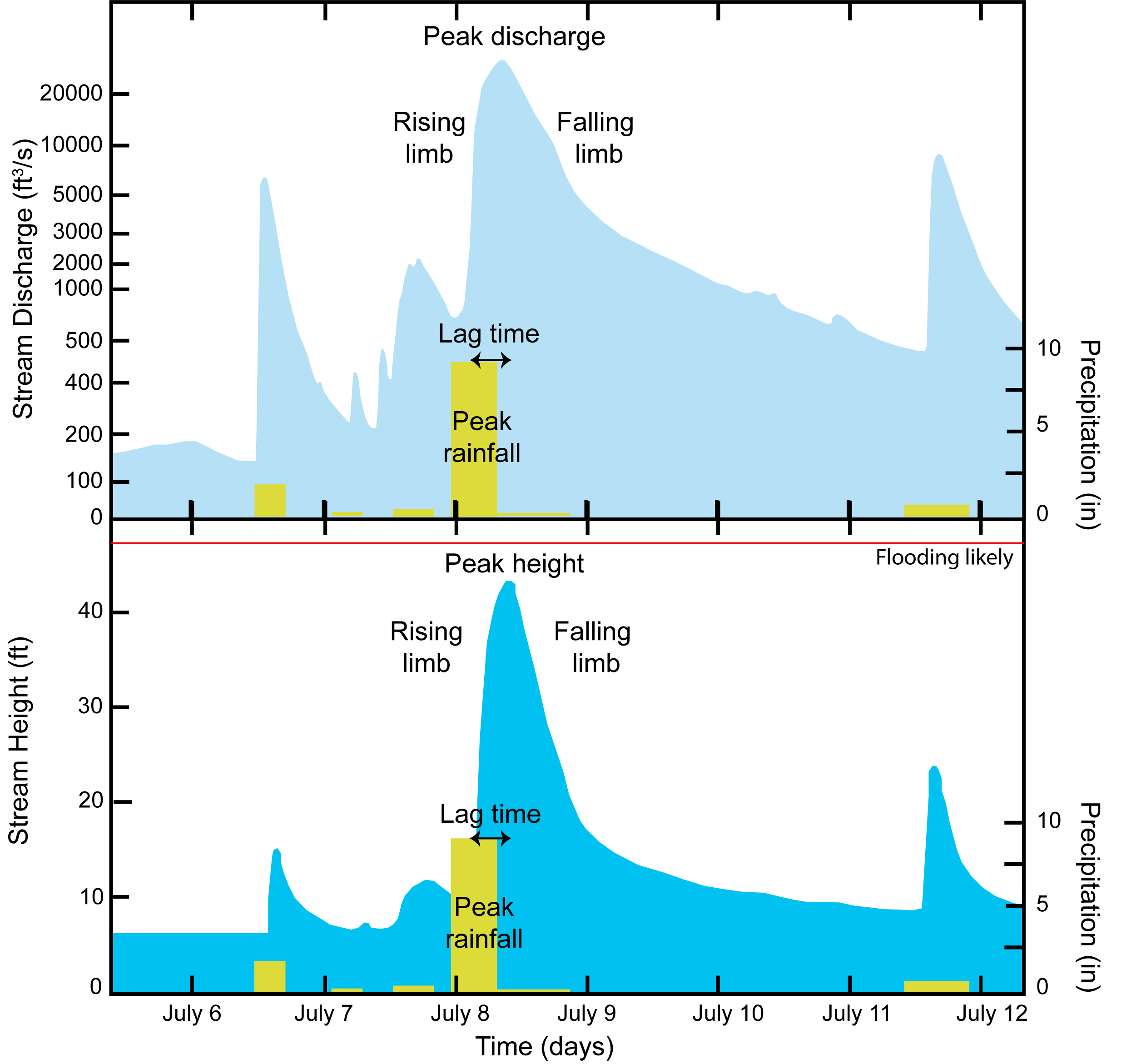
One of the results of a stream gauge is a hydrograph, a line graph that depicts water discharge over time for a cross-section within a stream and can show how stream discharge changes following a storm event. Discharge is the volume of water moving through a stream per unit time. In the U.S., discharge is commonly given as cubic feet per second (cfs). A storm hydrograph typically has time on the X-axis and discharge on the Y-axis (Figure 6.6). Sometimes, a secondary Y-axis for precipitation is shown. Time typically extends from several hours before a storm event to several hours beyond when the river returns to baseflow conditions. Discharge and precipitation are usually determined remotely using automatic gauging stations.
Exercise 6.6 – Create a Hydrograph
Now, let’s investigate some stream gauge data for two different streams.
- Table 6.3 contains precipitation and discharge data for two streams. Plot this data on a single graph. The Y-axis should range from 0 to slightly greater than the maximum values (e.g., if the maximum discharge is 1,382 cfs, the Y-axis range should be 0 – 1,400 cfs). Plot discharge on the Y-axis on the left side of the graph; plot precipitation on the Y-axis on the right side. Use bars for precipitation. You should use different colours for each data set.
- What is the lag time for Station A? ____________________
- What is the lag time for Station B? ____________________
- What is the peak discharge for Station A? ____________________
- What is the peak discharge for Station B? ____________________
- How do the receding limbs on the hydrograph for the two stations compare?
- One of these stations is in metropolitan Houston, while the other is in a rural area outside the city limits. Assuming watershed size is equal, which station is more likely to be the one in Houston (A or B)? How can you tell? Hint: Consider how lag times might differ in a city versus the countryside.
| Time | Precip. (in) | Station A Discharge (cfs) | Station B Discharge (cfs) |
| Noon | 1298 | 765 | |
| 3:00 PM | 1291 | 768 | |
| 6:00 PM | 1287 | 756 | |
| 9:00 PM | 1293 | 791 | |
| Midnight | 1297 | 772 | |
| 3:00 AM | 1299 | 758 | |
| 6:00 AM | 1295 | 764 | |
| 9:00 AM | 1297 | 782 | |
| Noon | 0.5 | 1376 | 2845 |
| 3:00 PM | 0.6 | 1456 | 3988 |
| 6:00 PM | 1.1 | 2245 | 5882 |
| 9:00 PM | 0.8 | 2578 | 6667 |
| Midnight | 0.6 | 2897 | 5058 |
| 3:00 AM | 3218 | 3982 | |
| 6:00 AM | 3456 | 2791 | |
| 9:00 AM | 3877 | 2362 | |
| Noon | 4168 | 2023 | |
| 3:00 PM | 3935 | 1676 | |
| 6:00 PM | 3812 | 1348 | |
| 9:00 PM | 3634 | 1201 | |
| Midnight | 3502 | 1032 | |
| 3:00 AM | 3371 | 967 | |
| 6:00 AM | 3013 | 903 | |
| 9:00 AM | 2878 | 854 | |
| Noon | 2615 | 827 | |
| 3:00 PM | 2467 | 792 | |
| 6:00 PM | 2271 | 788 | |
| 9:00 PM | 2119 | 781 | |
| Midnight | 2032 | 783 | |
| 3:00 AM | 1964 | 789 | |
| 6:00 AM | 1849 | 782 | |
| 9:00 AM | 1792 | 778 | |
| Noon | 1706 | 780 |
Additional Information
Exercise Contributions
Lab 6: Why Do The Red and Assiniboine Rivers Look Like They Do? was modified by Jessica Kristof and Ricardo L. Silva from the original Chapter 12: Rivers by Michael Comas, Lisabeth Arellano, Virginia Sisson, and Daniel Hauptvogel in Hauptvogel et al., (2024) and the original Lab 6, 7, 8: Surficial Processes in Ferreira and Young (2018).
References
Ferreira, K. and Young, J. (2018). GEOL 1340 The Dynamic Earth Lab Manual. Winnipeg, MB: Department of Geological Sciences, University of Manitoba
Hauptvogel, D., Sisson, V., and Comas, M. (2024). Investigating the Earth: Exercises for Physical Geology. Houston, TX: UH Libraries
