7.1 What is Geomorphology?

Geomorphology (from Ancient Greek: geo “earth”; morphe, “form”; and logos, “study”) is the scientific study of the origin and evolution of topographic and bathymetric features generated by physical, chemical, or biological processes operating at or near Earth’s surface. Geomorphologists seek to understand why landscapes look the way they do, to understand landform and terrain history and dynamics, and to predict changes through field observations, physical experiments, and numerical modelling.

Many forcing agents control the shapes of landscapes, with streams being the dominant force in most continental regions. Other forces include gravity, wind, glaciers, oceans, wildfires, people, and even water beneath the surface. Also important is climate – more about that in Chapter 10.

7.2 Desert Landscapes

The first landscape to explore is the desert, which is mainly affected by wind, and large sand dunes are a common feature. Desert sand dunes commonly form when there is an abundant sediment supply, and wind is strong enough to transport the sand. Dunes form where a dry climate prevents vegetation from interfering with their development. Sand dunes, however, are not restricted to deserts and can be found along seashores, along streams in semiarid climates, in areas of glacial outwash, and where sandstone bedrock disintegrates to produce an ample supply of loose sand.

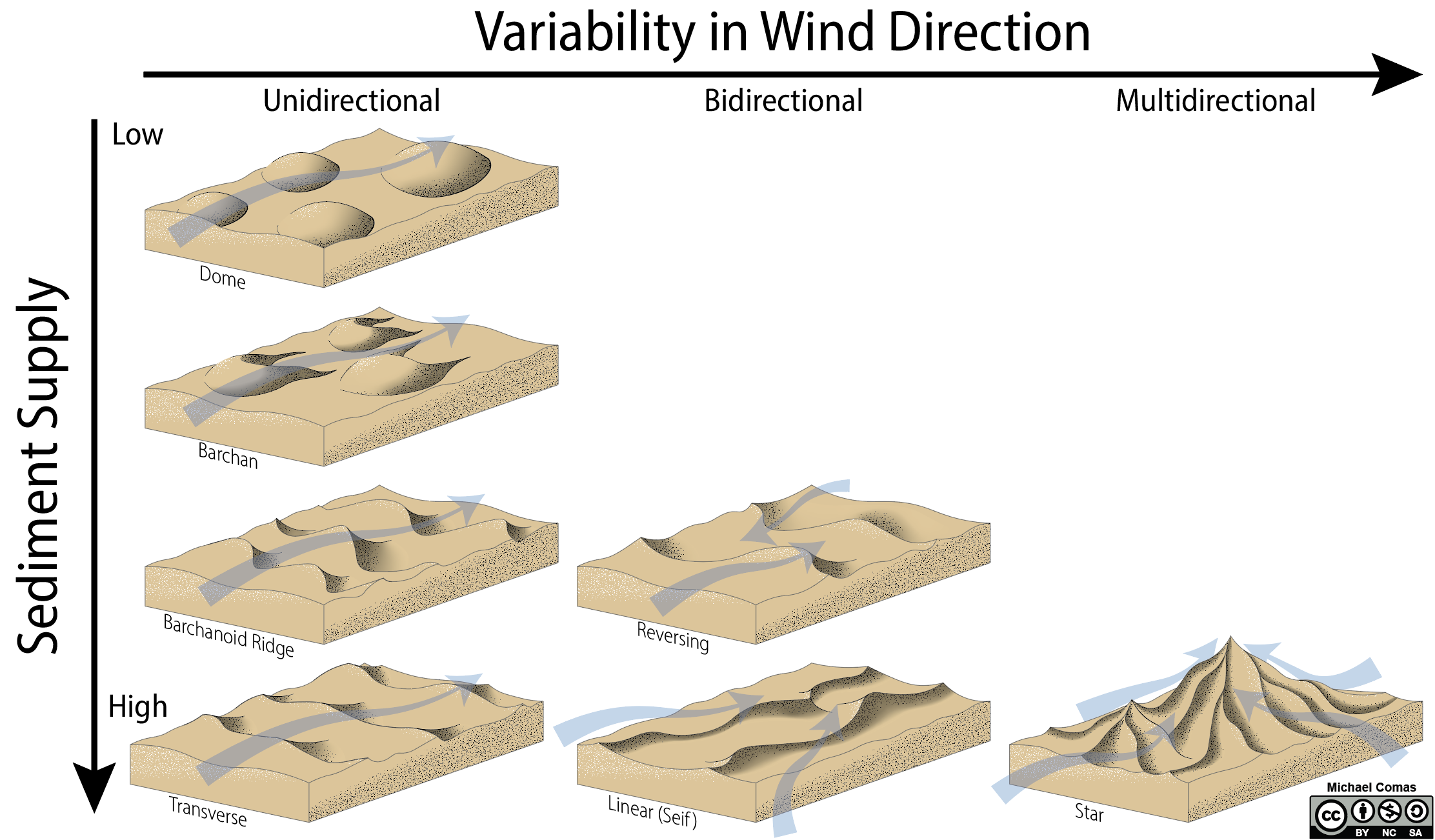
Two main factors dictate dune shapes: the amount of loose sediment and whether there is one or more prevailing wind directions. The strength, direction, and persistence of winds help determine how dunes develop. In some areas, winds will blow in one direction during the summer and another in winter. In other areas, there may be multiple wind directions. This variability in wind changes the shape of the dunes as well as their names (Figure 7.1). Sand is pushed or bounces (saltation) up the shallow side and then slides down the steep side (slip face). This characteristic shape is easy to see from a side view but harder to see in map view.

Vegetation acts as a barrier to wind, so sand may build up behind the vegetation. Vegetation also makes the sand surface rougher, which can affect sand movement. Also, deep roots can stabilize sand and prevent it from moving. These effects significantly impact sand dunes along the coast and at the edge of a desert where there is enough moisture for plants to grow.

Exercise 7.1 – Observing Sand Dunes

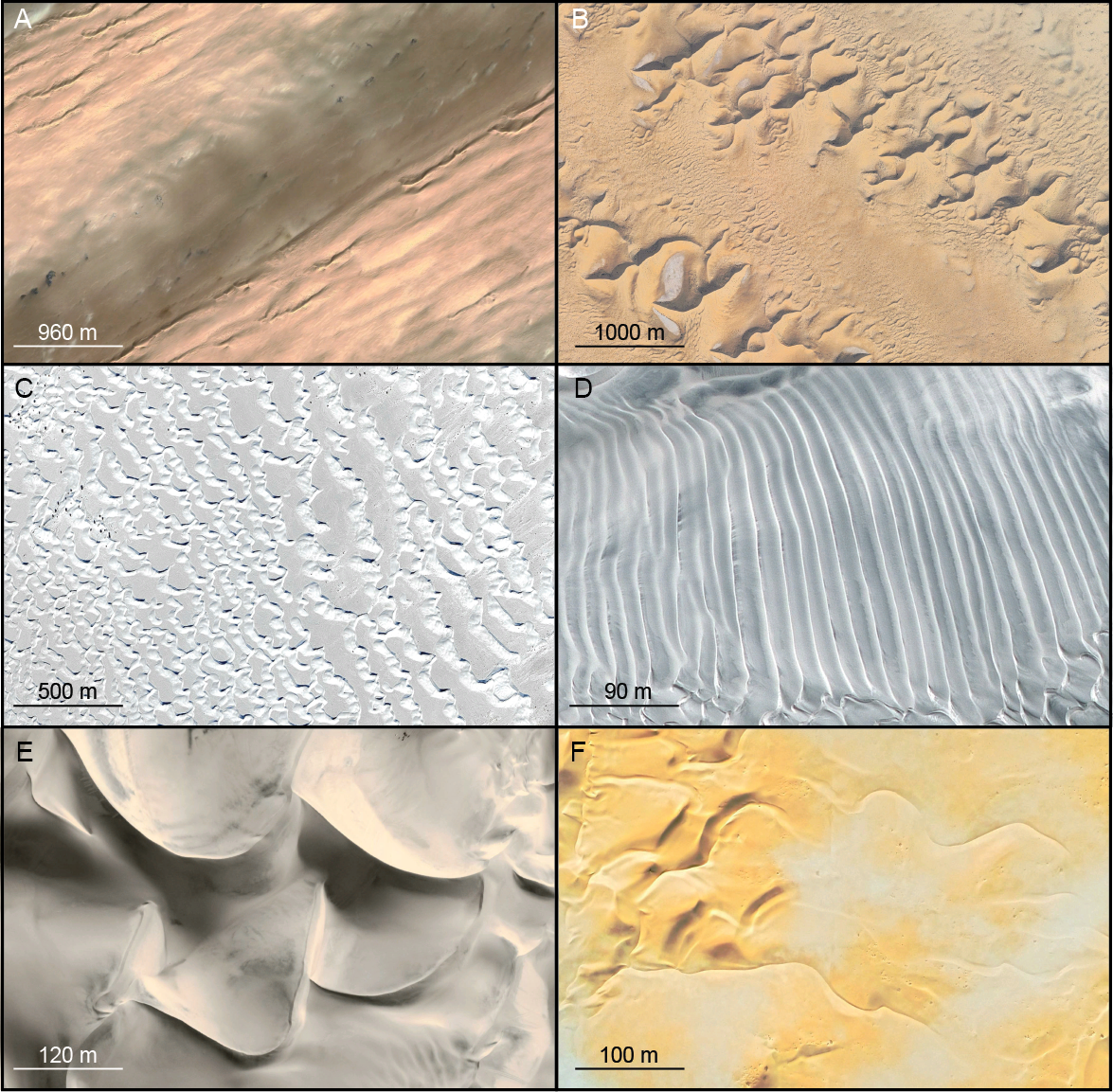
Figure 7.2 shows different types of sand dunes. Answer the following questions about them, and be sure to look at the scales on each image to get a sense of their size.

1. Observe the similarities and differences between the dunes in each photo. Trace the crest of as many dunes as possible.
2. For each image, describe the geometry of the dunes.
   1. Tenere Desert, Niger:
      

      ---

      ---

   2. Gran Desierto, Mexico:
      

      ---

      ---

   3. White Sands National Park, NM:
      

      ---

      ---

   4. Caravelli, Peru:
      

      ---

      ---

   5. Huachachina, Peru:
      

      ---

      ---

   6. Wadi Al Hajaa, Libya:
      

      ---

      ---

3. On each image, draw arrows to indicate the wind direction(s). Some may have more than one prevailing wind direction.
4. List the dunes in order of increasing sediment supply. Explain.
   

   ---

   ---

5. What do you think gives the sands of White Sand Dunes National Park their colour?
   

   ---

   ---

6. Do you notice vegetation in any of these arid settings?
   

   ---

   ---

7. How do you think vegetation affects dune formation?
   

   ---

   ---

8. Critical Thinking: Why can dunes vary in shape at different scales?
   

   ---

   ---

   ---

    

7.3 Glacial Landscapes

Next, let’s explore glacial landscapes where snow turns into dense glacial ice. A glacier is a body of ice that moves under its own weight.  Currently, glacial ice covers about 10% of Earth’s land surface, mainly in Antarctica and Greenland. At various times throughout geologic history, glacial ice has been much more extensive, covering up to 90% of the Earth’s land surface. They are the largest repository of freshwater on Earth (~69% of all freshwater) and are highly sensitive to climate change. For mountainous regions, glaciers are an important source of drinking water.

There are two types of glaciers: alpine (found at high altitudes) and continental (found at high latitudes). The largest glaciers can cover entire continents and be several kilometres thick. Ice masses of this size leave behind very distinct features. As they advance, they carve through the surrounding landscape and transport sediment. As they retreat, large volumes of meltwater carry and deposit sediment. These carved or deposited features can tell scientists that a glacier used to cover an area and inform them about how the glacier behaved.

Many glacial features are very large, larger than what can be observed in a single outcrop. One way that geologists can interpret large-scale landscape features is through LiDAR imaging (Light Detection and Ranging). LiDAR is an imaging technique that can make a detailed elevation map of an area without tree cover.

Isostasy and Glacial Rebound

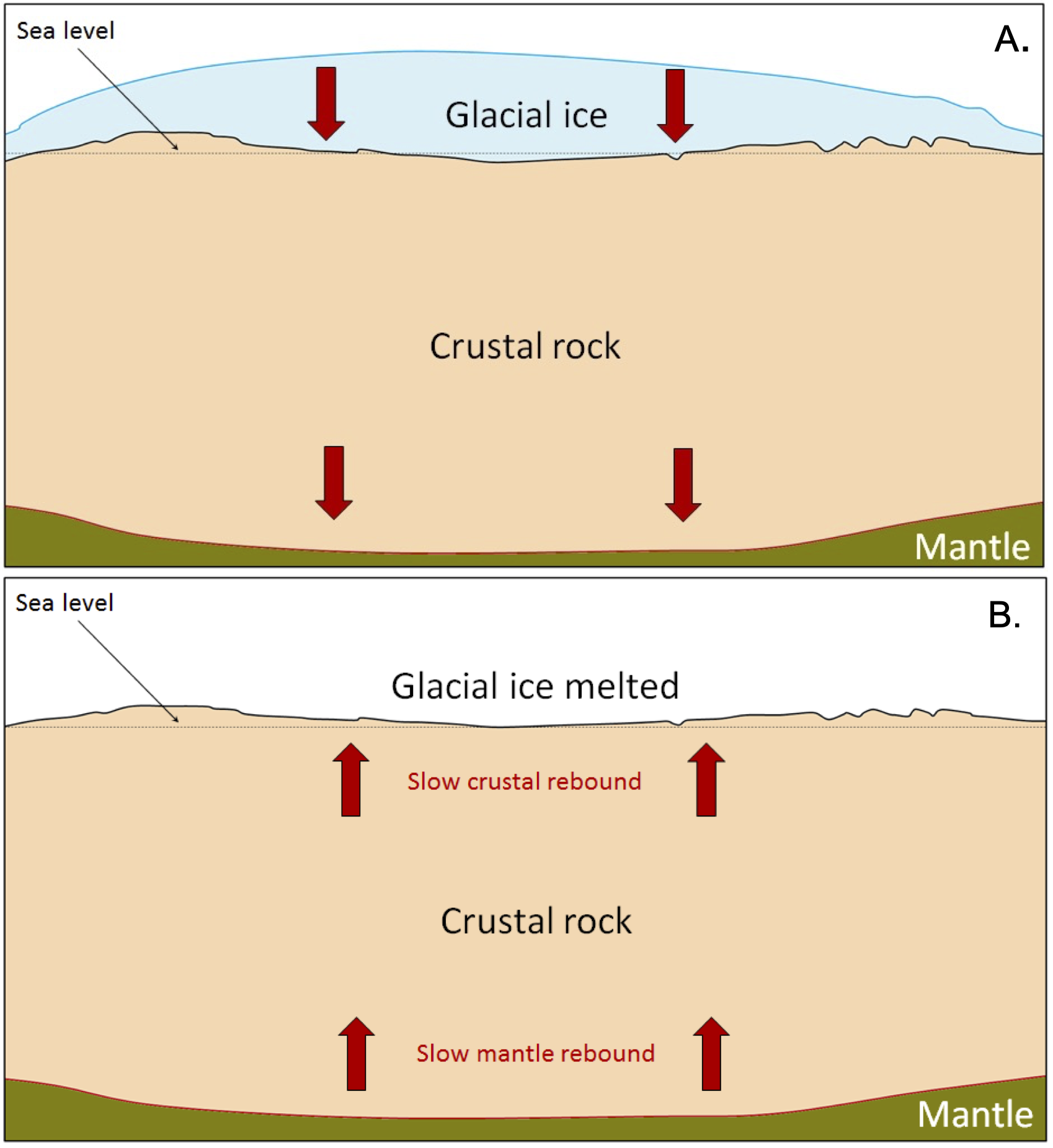
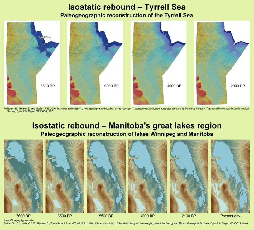
Another factor in understanding landscapes is the height of a region. In lecture, you may have been introduced to the concept of isostasy, or the principle that the Earth’s crust is floating on the mantle, like a raft floating in the water. Isostasy also applies to high topography in mountainous regions. As erosion reduces the height, the weight of the crust decreases, and it rebounds. This same principle applies to glaciers, as thick glacial ice adds weight to the crust and causes the crust to subside. For example, the Greenland Ice Sheet is over 2,500 m thick, and the crust beneath the thickest part has been depressed to the point where it is below sea level over a wide area (Figure 7.7). The same is true in parts of Antarctica. When the ice sheet melts, the crust and mantle will rebound, as it has happened in Manitoba over the last thousands of years.

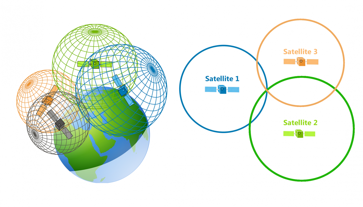
To measure Earth’s movements, geoscientists use high-precision global positioning system (GPS) instruments. You probably have used the GPS in your mobile phone to get where you want to go. Most of the time, you don’t have to pay attention to the vertical data from the GPS unless you are on a hike and need to know if you are at the correct elevation. So, how does the GPS get elevation data? A GPS uses trilateration to determine its location. This uses overlapping spheres instead of overlapping circles to determine location (Figure 13.8). In general, the more satellite data, the more precise and accurate your location will be calculated.

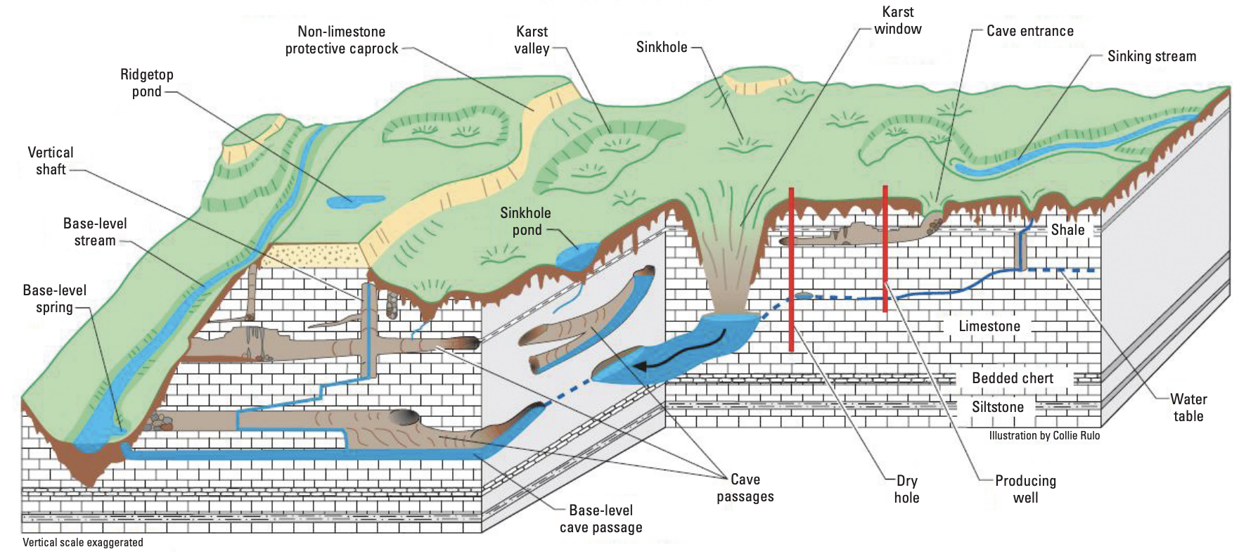
7.4 Groundwater, Karst, and Subsidence

It may not seem like an important part of the landscape, but groundwater flow controls many aspects of geomorphology underground. Caves are a geomorphic feature formed beneath the surface by the dissolution of limestone. Limestone at the Earth’s surface can dissolve to form karst topography. Both caves and karst form as carbon dioxide from the atmosphere dissolves in rainwater, making the water slightly acidic. The acidic water widens existing cracks or crevices, which leads to even larger cracks and more water flow and dissolution. In addition to chemical weathering, mechanical erosion occurs as loose rock fragments transported by water erode the sides of the openings.

A critical requirement for the development of karst is water. Without water, there would be no karst or caves. On a global scale, a significant portion (15-20%) of the Earth’s surface is underlain by limestone that has the potential to form karst. Therefore, understanding karst processes is important, particularly where humans interact with this landscape (Figure 7.11). Karst landscapes have features and resources that are not present in non-karst landscapes. Karst aquifers provide the main source of water; for example, 25% of US groundwater comes from karst, such as the Edwards aquifer in central Texas.

Exercise 7.3 – Karst and Sinkholes

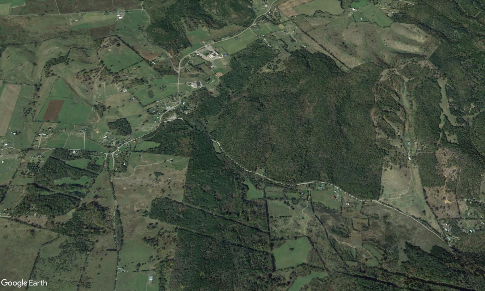
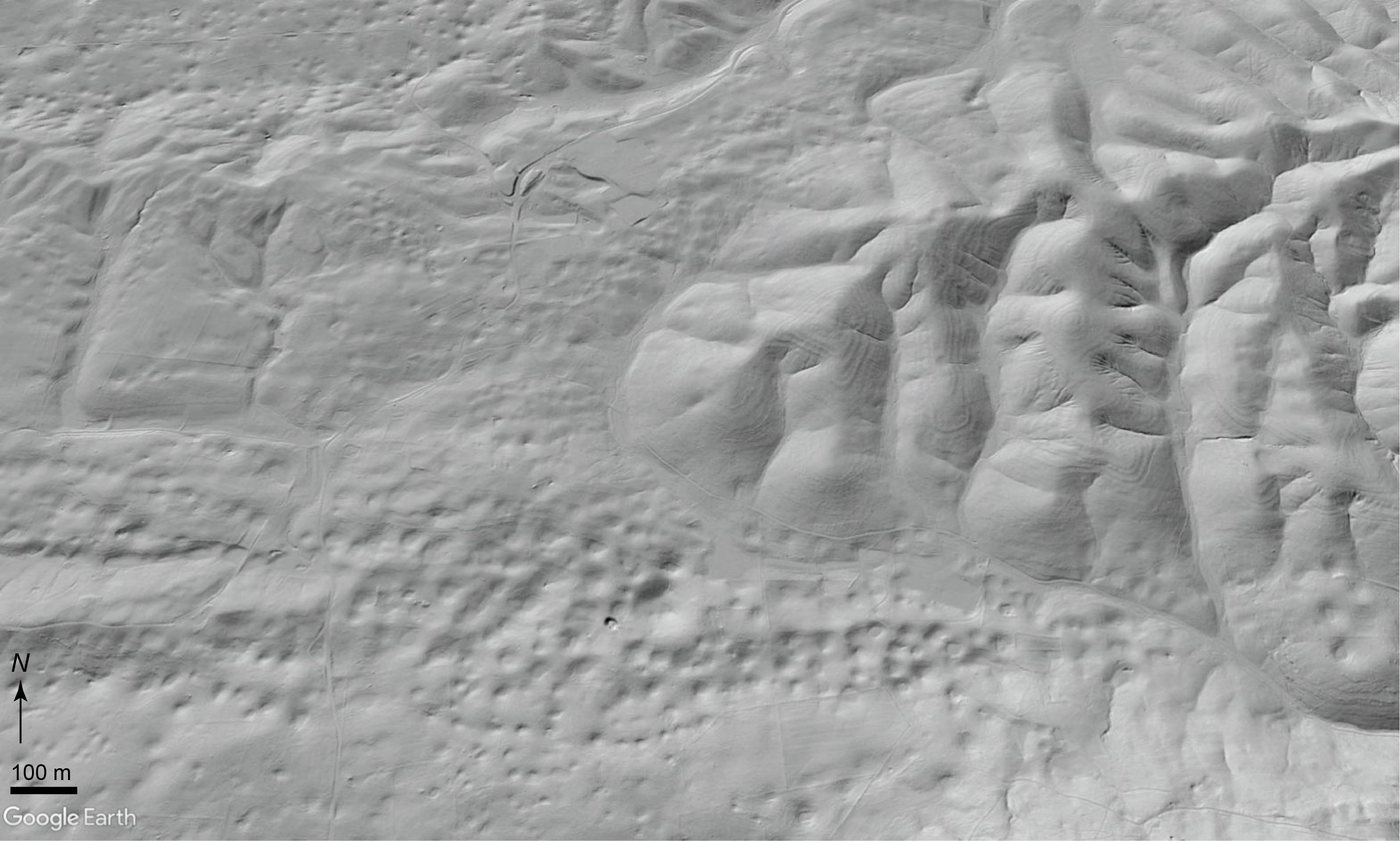
Extensive carbonate occurs in southern Virginia and northern Tennessee. There is a state park near Clinchport, VA, with a natural tunnel that is over 255 m (838 ft) long that once had a railroad running through it. Compare the satellite image (Figure 7.12) with the LiDAR image of the same area (Figure 7.13) for an area east of Natural Tunnel State Park.

1. Make observations about the landscape in the tree-covered area in the LiDAR.
   

   ---

   ---

2. Compare this with the farmland surrounding the wooded area. Use Figure 7.13 and name the landforms in the farmland.
   

   ---

   ---

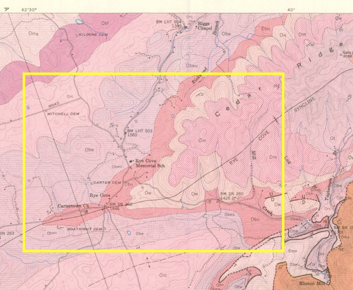
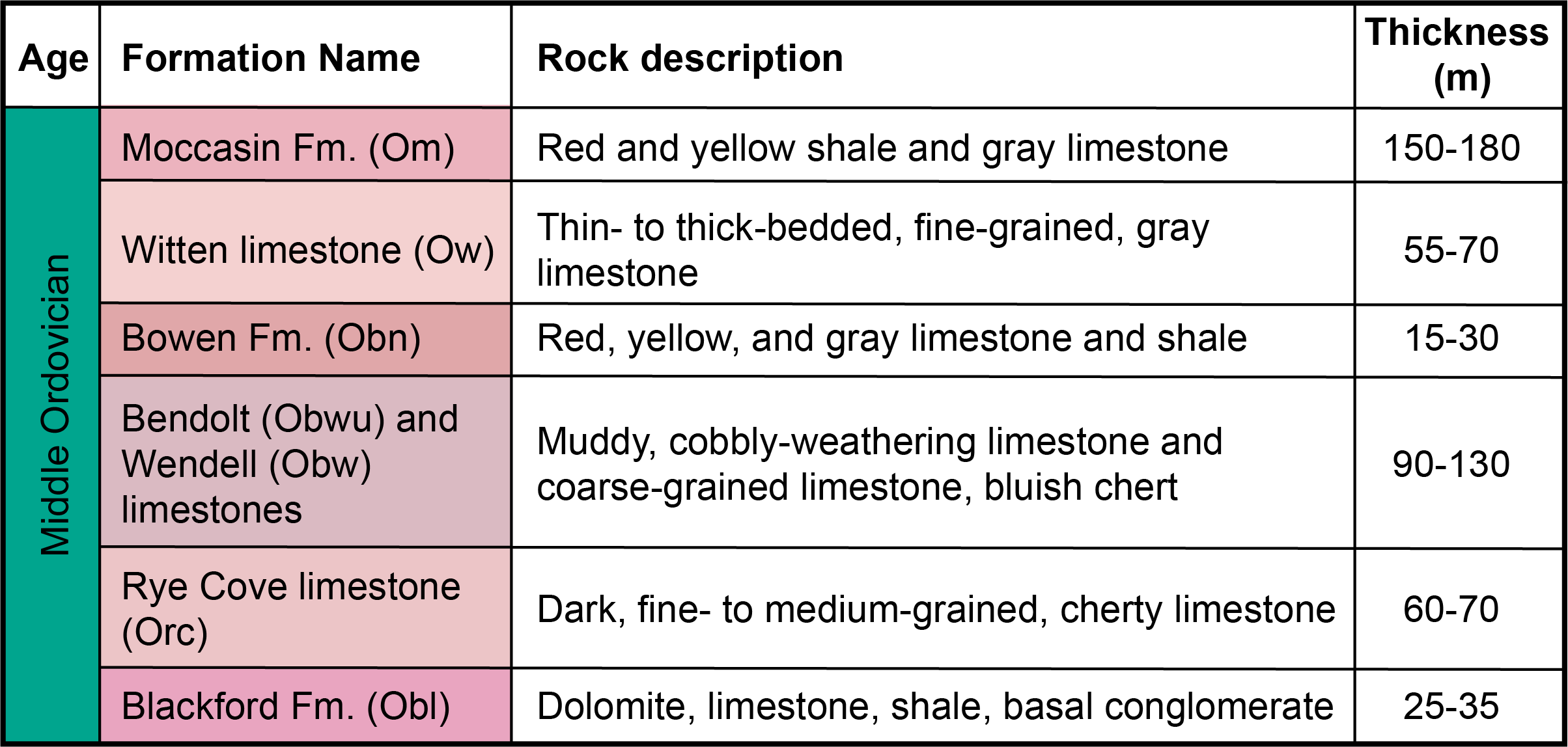
3. Use the geologic map and rock descriptions in Figures 7.14 and 7.15 and list the different geologic units in each area.
   

   ---

   ---

4. Critical thinking: Almost every unit in this area is a type of limestone. Why is some of the area filled with sinkholes, and some does not have any karst features?
   

   ---

   ---

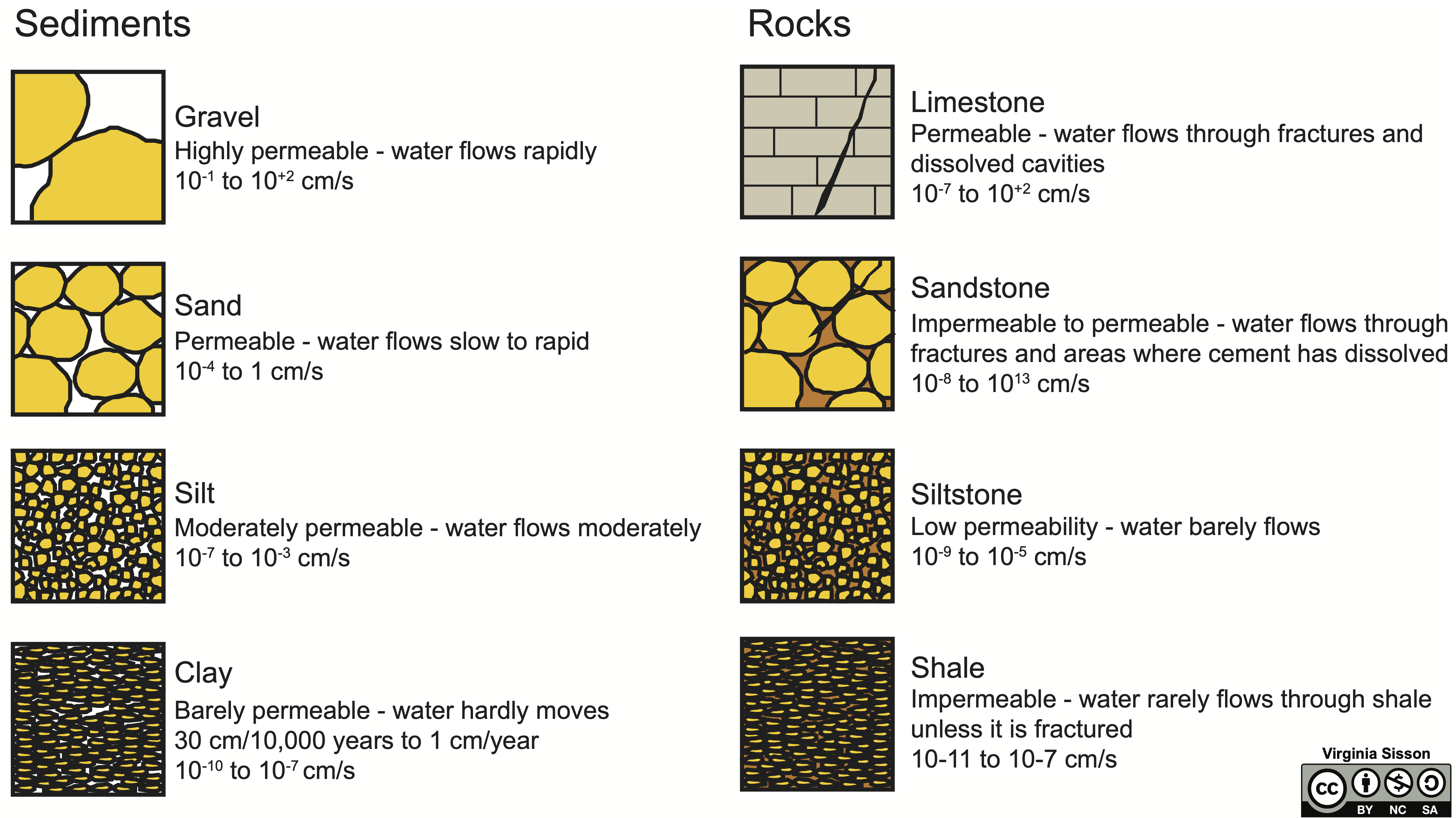
Both surface water and groundwater play a significant role in landscape development. Groundwater is stored in the open spaces within rocks and within unconsolidated sediments. Porosity is the percentage of open space between grains in a sediment or sedimentary rock. Some volcanic rocks have a special type of porosity related to vesicles, while some limestones have extra porosity related to cavities within fossils.

Do you think water can flow through basalt with lots of vesicles? No, as there is another parameter, permeability, which is the most important variable in groundwater. Permeability describes how easily water can flow through the rock or unconsolidated sediment and how easily it will be to extract the water for our purposes. A permeable material has a greater number of larger, well-connected pore spaces, whereas an impermeable material has fewer, smaller pores that are poorly connected. The characteristic of permeability of a geological material is quantified as the hydraulic conductivity (K) measured in centimetres per second.

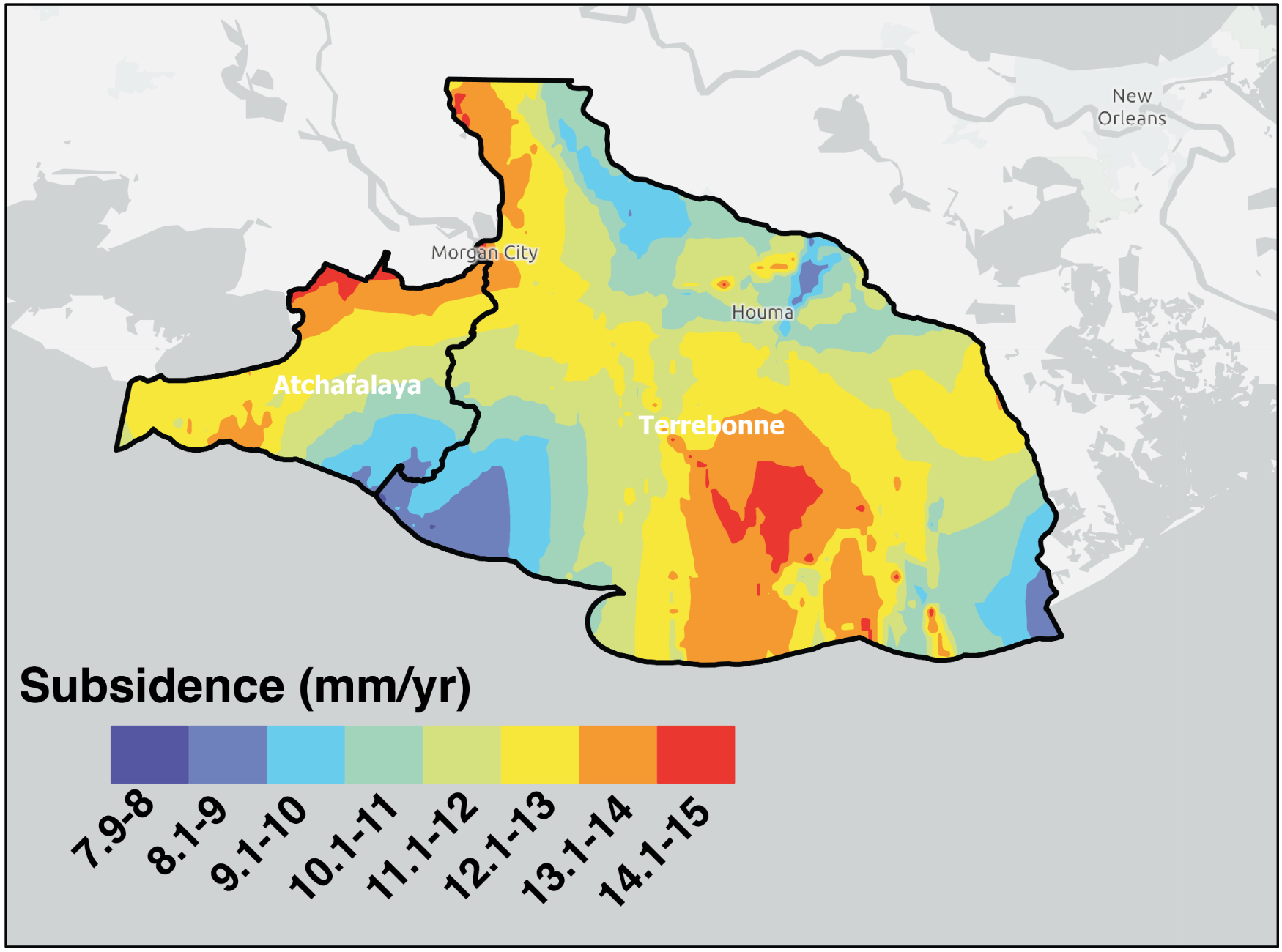
Subsidence may seem like a minor change in the landscape because, in most areas, sinking is negligible. To those living near the coast, it’s a major threat, compounded by rising sea levels and climate change. Not only will coastal communities be affected, but their water supplies are also susceptible to an influx of saltwater. This problem makes many more vulnerable to sea level changes, such as the Mississippi Delta and American Samoa. This process results in coastal retreat and land loss. In the Mississippi Delta, about 60 km²/year is vanishing. Not only is this important for those who live there, but the Atchafalaya River basin (Figure 7.18) provides flood relief for the Mississippi River, slowing its flow and trapping nutrients and pollution, improving water quality as it flows into the Gulf of Mexico.

Exercise 7.4 – Groundwater Flow

Your instructor will provide you with four maps to complete the following questions. These maps include:

1. Bedrock Geology (Plate 7)
2. Potentiometric Surface of the Upper Carbonate Aquifer – Sept 1980 (Plate 12)
3. Upper Carbonate Aquifer Chloride Ion Content for 1980 (Plate 16)
4. Waste Disposal Sites (Plate 8)

These maps are Geological Engineering Maps of Winnipeg (1983). These thematic maps are part of a preliminary report assessing Winnipeg area development sites, with a focus on building foundations and groundwater conditions. The maps provide information to help avoid land use conflicts and assist in planning detailed site investigations before development. In 1984, approximately 90 commercial wells operated in the City of Winnipeg. Most wells supply water for commercial and industrial cooling, although some groundwater is used in heating systems, market garden irrigation, or domestic water supplies in suburban fringe areas. In 1980, groundwater accounted for about 15% of all water consumption in Winnipeg.

1. Use Bedrock Map (Plate 7). What is the name and lithology (i.e., rock type) of the carbonate bedrock that contains the aquifer underlying the University of Manitoba Fort Garry campus?
   

   ---

   ---

   ---

2. Use Plate 12 and Figure 6-4. Maps showing the water levels (whether the aquifer is confined or unconfined) are called potentiometric surface maps. You drew a potentiometric surface map in Question b. The contours on Plate 12 (and Fig. 7.19) represent the elevation (above sea level) of the water level, making these potentiometric surface maps. Plot about eight flow lines on Figure 7.19 to indicate the direction of groundwater flow in the Winnipeg area. (One is plotted on the map for you already.)
   

   ---

   ---

3. Use Upper Carbonate Aquifer Chloride Ion Map (Plate 16). Why can’t a well located in the southwest quadrant of the city produce good quality water for domestic use?
   

   ---

   ---

   The main landfill site in southern Winnipeg is the Brady Road Landfill Site. (Use Plate 8 to find its location.)

4. If waste were to leak from the landfill into the Upper Carbonate Aquifer, in which direction would the waste plume flow?
   

   ---

   ---

5. Using the Potentiometric Surface Map of the Upper Carbonate Aquifer (Plate 12), determine the hydraulic gradient between the northeast corner of the Brady Road Landfill Site and the control well at the University of Manitoba. Express your answer as a percentage.
   

   ---

   ---

   The surficial deposits in & around the University of Manitoba consist of a relatively thick, upper sequence of clays that Glacial Lake Agassiz deposited. These are underlain by about 1 metre of thickness of glacial till, which in turn, overlies solid bedrock. Determine the length of time (in years) it would take groundwater to move from the Brady Road Landfill Site to the University of Manitoba Control site through (a) Lake Agassiz clay deposits and (b) glacial till. Use the hydraulic conductivity values given below.

   ---

1. Unit                                                              Hydraulic conductivity Lake Agassiz clay deposits                       2.06 x 10-9 m/sGlacial till                                                     1.50 x 10-7 m/s(Hint: Note that hydraulic conductivity is an expression of distance divided by time. You will measure the distance from Plate 8. Now solve for time. The algebraic expression is simple – the only difficult part of this question is managing unwieldy numbers. Convert seconds into a more sensible unit of measure – in this case, years.)

 

Additional Information

Exercise Contributions

Lab 7: Why Is Manitoba So Flat? was modified by Jessica Kristof and Ricardo L. Silva from the original Chapter 13: Landscapes by Virginia Sisson, Daniel Hauptvogel, Xiao Yu, and Michael Comas in Hauptvogel et al., (2024) and the original Lab 6, 7, 8: Surficial Processes in Ferreira and Young (2018). 

References

Brent, W.B., 1963, Geology of the Clinchport quadrangle, Virginia, Virginia Division of Mineral Resources Report of Investigations 5, 47 pp., Map Scale: 1:24,000

Chowdhury, A.H. and M.J. Turco, 2006, Chapter 1, geology of the Gulf coast aquifer, Texas. In R. E. Mace, S. C. Davidson, E. S. Angle, & W. F. Mullican (Eds.), Aquifers of the Gulf Coast of Texas (Vol. 365, pp. 23–50). Austin, Texas: Texas Water Development Board. Report.

Ferreira, K. and Young, J. (2018). GEOL 1340 The Dynamic Earth Lab Manual. Winnipeg, MB: Department of Geological Sciences, University of Manitoba

Freeze, R.A. and J.A., Cherry, 1979, Groundwater, 604 pp. CC-NC available as pdf

Hauptvogel, D., Sisson, V., and Comas, M. (2024). Investigating the Earth: Exercises for Physical Geology. Houston, TX: UH Libraries

McKee, E.D., 1979, A study of global sand seas, U.S. Geological Survey Professional Paper 1052 https://doi.org/10.3133/pp1052

Taylor, C.J. and E.A. Greene, 2008, Hydrogeologic Characterization and Methods Used in the Investigation of Karst Hydrology, in Field Techniques for Estimating Water Fluxes Between Surface Water and Ground Water, Edited by D.O. Rosenberry and J.W. LaBaugh, U.S. Geological Survey Techniques and Methods 4–D2, 128 pp.

Varugu, B., and C. Jones, 2023. Delta-X: Land Subsidence Rate, Mississippi River Delta (MRD), Louisiana, USA. Oak Ridge National Laboratory Oak Ridge National Laboratory (ORNL) Distributed Active Archive Center (DAAC), Oak Ridge, Tennessee, USA. DOI: 10.3334/ORNLDAAC/2307